
http://dx.doi.org/10.15649/2346030X.787
Velocity Profile of a Ferrofluid in the Presence of Rotating Magnetic Fields. Pseudo-Analytical and Numerical Solutions.
Cristian Camilo Jiménez-Leyva1
Hermann Raúl Vargas-Torres2
Carlos Rodrigo Correa-Cely3
-
Universidad Industrial de Santander, Colombia. E-mail: cristian.camilo.jimenez@gmail.com Autor de correspondencia
- Universidad Industrial de Santander, Colombia.
Received: May 9th 2020.
Aprobado: August 9th 2020.
Atribución 4.0 Internacional (CC BY 4.0)
Abstract— From the beginning of ferro-hydrodynamics, several authors have proposed analytical models to describe the movement of ferrofluids in the presence of rotating external magnetic fields. To this effect they have made valid simplifications in certain and very restricted physical situations. In this work we analyze the effects of these approaches against numerical solutions that do not make use of them. A sample of ferrofluid immersed in containers with three types of geometries was considered: one of flat and parallel plates, one cylindrical and another coaxial cylindrical. Velocity profiles were obtained by these two strategies. The analytical solution leads to a linear model with several simplifications, while the second, numerical in nature, generates a non-linear model, but without approximations. The simulation results showed that the simplifications made in the analytical strategy generate profiles that are valid only for magnetic field intensities lower than the respective ferrofluid saturation values. Additionally, and given the level of development of analytical modeling, it was found that the numerical solution is currently the most appropriate to evaluate the ferro-hydrodynamic model, since it does not have restrictions related to the intensity of the magnetic field. In the same way, it allows to evidence the phenomenon of saturation in the velocity profiles by increasing the intensity of the magnetic field, a situation observed experimentally, and unpredictable by means of these currently available pseudo-analytical solutions.
Keywords: Ferrofluid, Pseudo-analytical solution, Rotating magnetic fields, Velocity profile.
The phenomenon of a ferrofluid flow contained in a square, cylindrical and annular geometry has been studied in recent years [1-5], in order to explain the causes of velocity profiles resulting from the presence of an External Rotating Magnetic Field (ERMF). However, no consensus has been reached at the time of determining the generators of the movement, and various theories have been postulated [4,6-13] without having been able to describe or predict the experimentally measured profiles so far. One of the theories that was discarded years ago, but that has recently gained relevance due to flow measurements in the internal parts of the ferrofluid [14], has been the Internal Angular Momentum Diffusion Theory (IAMDT) which, as its name implies, attributes the flow to the diffusion of internal angular momentum from the magnetic nanoparticles to the carrier fluid, [3,4,6,11-13]. In this hypothesis, the vorticity between the fluid layers differs from the spin velocity of nanoparticles, which are rotating by the action of a magnetic torque generated by the difference in the direction of the ERMF and the magnetization of the ferrofluid [3]. Although IAMDT qualitatively corresponds to the measured profiles, there are obvious quantitative differences between theoretical and experimental profiles that continue to disqualify it as a tool capable of describing flow profiles, [15]. One cause of this situation is the limitation of the pseudo-analytical solution of the model. This restricts the validity of the velocity profiles obtained using ERMFs of very low amplitude and frequency [11-13, 16], which differs from the experimental conditions in which measurements have been made [15]. Therefore, a model solution strategy is required in which such simplifications are not demanded [5]. With this, it would be possible to eliminate the restrictions that prevent an adequate evaluation of the IAMDT's performance in the prediction of ferrofluids velocity profiles under the effect of ERMFs of various amplitudes and frequencies. In this vein, this article compares the profiles obtained through an approximate model (pseudo-analytical solution) and another without approximations (numerical solution algorithm), to evaluate the effect of these restrictions, observing the differences and limitations of the resulting profiles.
This model compiles the IAMD theory, which in turn includes the hydrodynamic equations for the generation of velocity profiles, and the magnetic equations, which describe the applied rotating magnetic field, as well as the magnetization of the ferrofluid. We disaggregate each one of them below.
-
Hydrodynamic equations
The hydrodynamic system is composed of the continuity equation for incompressible fluids (Eq.(1)), the linear momentum balance equation (Eq.(2)), and the internal angular momentum balance equation (Eq.(3)). This set of equations expressed in a dimensionless form is [4,11-13,17]:

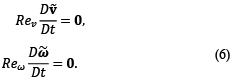
where v ̃ is the average linear velocity vector of the ferrofluid, D/Dt the material derivative, ζ the parameter of the vortex viscosity, η the shear viscosity, Ω ̃=Ω τ the parameter that relates the rotational velocity of the ERMF and the magnetization relaxation constant, M ̃ ferrofluid magnetization, H ̃ ERMF intensity, p ̃ the absolute pressure of the system, ω ̃ the average angular velocity of the magnetic nanoparticles, η_e=η+ζ without any physical significance, κ=((4ηζR_0^2)/(η'η_e ))^(1/2) parameter related to the coefficient of "spin viscosity" η^', responsible for the diffusion of Internal Angular Momentum in the fluid layers. On the other hand, ve=((4ηζR_0^2)/(λ'η_e ))^(1/2) is related to the volumetric coefficient of the “spin viscosity” λ^'. Finally, Re_v=(ρR_0^2)/η ((μ_0 χ_i K^2 Ω_f)/ζ) and Re_ω=ρI/ζ ((μ_0 χ_i K^2 Ω_f)/ζ) represent the translational and rotational Reynolds number respectively. The variables without dimensions of the system of ferrohydrodynamic equations of order one, and represented with the symbol ˜ at the top of these, are defined in Eq. (4) and (5) [4, 5, 11-13, 18].
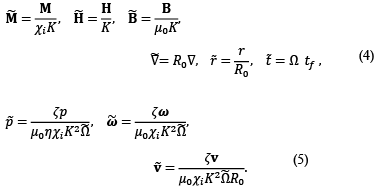
Likewise, χ_i represents the initial magnetic susceptibility of the ferrofluid, μ_0 the magnetic permeability of the air or vacuum, R_0 the radius of the container, t_f the analysis time of the flow phenomenon and K the peak value of the magnetic field strength. Now, analyzing the dynamics of the steady state system, an approximation is made based on the Reynolds number [19]. It assumes that diffusive effects predominate over inertial effects, so that in the phenomenon of flow generation it must be fulfilled that.
The boundary conditions used for the solution of the equations that describe the hydrodynamic problem are the non-slip and non-penetration conditions, for the linear velocity of the ferrofluid and the rotational velocity of the nanoparticles, as shown in Eq. (7) and (8) [3].
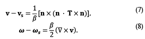
In Eq. (7) n is the normal unit vector, from the ferrofluid volume to the air phase of the interface, β is the friction coefficient dependent on the sliding velocity, v_s is the velocity at the walls and T is the Cauchy stress tensor in the fluid. ω_s is the angular velocity at the walls. Similarly, for the local average angular velocity of the particles, a boundary condition is proposed in which the possibility arises that the particle, near a solid surface, rotates at the same surface velocity, that is, β=0. On the other hand, in the literature they propose that through an interfacial momentum balance in a control volume, the boundary condition that must be met at the ferrofluid-air interface can be obtained, as in Eq. (9).
![]()
In this equation, C is the stress tensor, which is a measure of the transport of Internal Angular Momentum (IAM) by direct contact. Condiff and Dahler [20] proposed a constitutive equation for the torque stressor C, who assumed it as symmetrical and dependent only on the gradient of the rotation velocity ω.

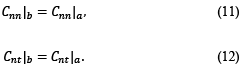
In addition, Eq. (9) shows that the pair of efforts is continuous throughout the interface, considering that a and b represent the two phases that are part of the interface of the system under study. Therefore, the normal and tangential boundary conditions, for the internal angular momentum, are obtained through the internal product of Eq. (9) with the normal and tangential unit vectors, n and t. In this way, the following valid relationships are available for any point of the ferrofluid-air interface [13].
Likewise, the literature reports that with Eq. (13) and (14) the following relationships can be established for the solution of the system of hydrodynamic differential equations.
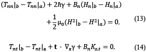
where T_nn and T_(nt )are the normal and tangential component of the stress tensor, respectively, which appear below.

In Eq. (13-16), ℏ represents the coefficient of curvature of the interface, ∇_s the surface gradient at the interface, γ the surface tension and K_s the surface current density. Additionally, in Eq. (13) it is taken into account that.

-
Equations describing the magnetic process
The system of magnetic equations has as one of its components the one related to the relaxation of magnetization. In the case where low amplitude rotary magnetic fields are applied, the magnetization equation of Shliomis [3,11,12,21] (Sh-72), Eq. (18) is used. Already for the case of flows in the presence of these fields but of high intensity, the magnetization equation of Martsenyuk, Raikher and Shliomis [22,23] (MRSh-74), Eq. (19) is used. It describes the behavior of the magnetization vector of the magnetic particle, in its attempt to align with the ERMF. In addition to these magnetic relaxation equations, the Maxwell equations, i.e., Ampère-Maxwell Law, Eq. (20), and Magnetic Field Gauss Law, Eq. (21), are used for the description of the rotating magnetic field present within the ferrofluid sample container.
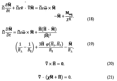
where ε=(μ_0 χK^2 τ)/ζ=2/3 α^2 is called the perturbation parameter, [11]. The constants of the parallel and perpendicular relaxation times B_∥and B_⊥, respectively, appear below.

Similarly, to model the phenomenon of magnetic saturation of the ferrofluid, the Langevin equation, Eq. (23) will be used.

In this equation, subscripts 1 and 2 correspond to the components of the magnetic field intensity vector. The Langevin parameter, α, that appears in it is defined as,

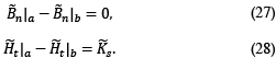
That being said, to determine if a ferrofluid is subjected to a high or low amplitude magnetic field, the value of the said Langevin α parameter is taken as a reference. If α≪1 implies a low intensity magnetic field. On the contrary, a value of α≫1 implies one of high magnitude. In the first case (α≪1), there is a linear relationship between the equilibrium magnetization M_eq and the intensity of the magnetic field H. In the second case M_eq is approximately equal to the saturation magnetization of the ferrofluid. Similarly, to define the frequency of the external magnetic field, the dimensionless parameter Ω ̃ is examined. Thus, a value of Ω ̃≪1 describes a low frequency magnetic field and vice versa, values of Ω ̃≫1 correspond to high frequencies. In relation to the boundary conditions for the magnetic problem, these are condensed into two equations, the continuity of the normal component of the magnetic field density B, and that corresponding to the jump of the tangential component of the magnetic field intensity H, expressed as follows.

where K ̃_s is the current distribution on the surface of the walls of the ferrofluid container. The scalar components of the interfacial magnetic boundary equations are.
-
Geometry of flat and parallel plates
The physical system consists of a rectangular container of width and height δ, with walls on the lower surface and two sides (x ̃=0, y ̃=0 y y ̃=1) and infinite length (z direction), as can be seen in figure 1. It also contains a ferrofluid, which in its free surface comes into contact with the surrounding air (ferrofluid-air interface at x ̃=1). The rotating magnetic field is generated by two alternating current transport coils, out of phase 90^( ^° ) electric and 90^( ^° ) in space. The present fields are generated in the axial direction of the channel (magnetic field generated by the current in the xy plane and counterclockwise, (see figure 1). They also appear in the direction of the yz plane (magnetic field generated by the flow symbolized through circumferences, where the x inside the circumference constitutes the flow that enters the xy plane, and the filled circumferences, represent the flow that leaves the xy plane. (See figure 1). The origin of the coordinate axis it is located in the lower left corner of the front view of the channel. It is assumed that the resulting magnetic field rotates on the xz plane, because of the electric current flowing through each coil and its physical arrangement. Consequently, it is intended to predict profiles of: 1) the average linear velocity of the fluid in the axial direction v ̃=v ̃_z (x ̃,y ̃ ) i_z and 2) the angular velocity of the nanoparticles at the points of the xy plane of the channel, that is to say, ω ̃=ω ̃_x (x ̃,y ̃ ) i_x+ω ̃_y (x ̃,y ̃ ) i_y, considering that M ̃ ·∇ ̃H ̃=0, due to the assumption of uniformity of the rotating field. Finally, it is assumed that the physical arrangement of the external current sources makes it possible to define the intensity and the magnetic field density such as H ̃_z (t ̃ )=sin(t ̃ ) y B ̃_x (t ̃ )=cos(t ̃ ), respectively.
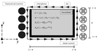
Figure 1: Diagram of the cross section of the rectangular channel and its associated variables for the application of IAMDT.
Source: Own elaboration.
III. METHODOLOGY OR PROCEDURES
-
Ferro-hydrodynamic equations, case α≪1
In order to obtain the solution to the system of differential equations of the hydrodynamic problem, a uniform ERMF was assumed, so that, M ̃ · ∇ ̃H ̃=0. Likewise, nullity was added in the divergence of the angular velocity of the nanoparticles, that is, ∇ ̃ ω ̃=0. Also, considering that there are no pressure differentials in the direction of the ferrofluid movement, you have to ∇ ̃p ̃=0. Finally, for the analytical solution the parameter η^'=0 was assumed, and therefore, κ→∞. Thus, the equations of hydrodynamic balance remain as:
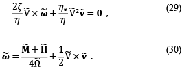
By replacing Eq. (30) in Eq. (29), the nullity of the Laplacian of the linear velocity vector is obtained.

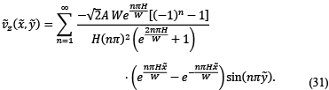
From Eq. (30) - (31) the linear velocity profiles are obtained, implementing the Fourier series (SF) method, for a channel of width W and height H. Resulting in Eq. (32) [5, 24].
- Ferro-hydrodynamic equations, case α≫1
For magnetic fields of intermediate or high intensity, the linear momentum balance equation remains the same, while the amount of IAM, bearing in mind Eq. (6), becomes.
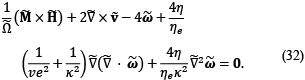
Considering the coordinates in which IAM is presented (x and y coordinates), the respective component equations are (η^'≠0) [5].

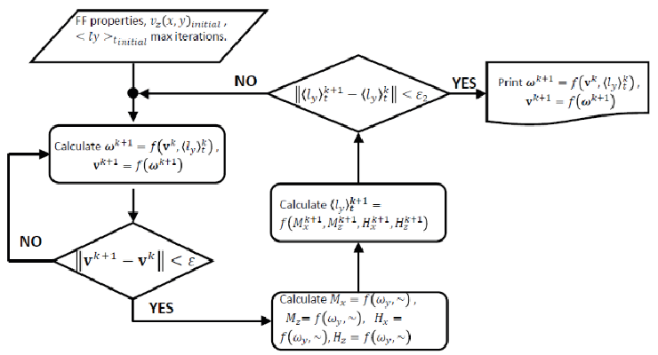
Figure 2: Flowchart of methodology implemented in the development of the numerical algorithm, for the solution of the IAMDT ferrohydrodynamic problem.
Source: Own elaboration.
For their solution, these equations are discretized taking into account the presence of high intensity magnetic fields (α≫1) and the transmission of IAM (η^'≠0) [5]. In this order of ideas, the flow chart
corresponding to the methodology implemented for the numerical solution of the ferrohydrodynamic model is presented in Figure 2. First, the methodology initializes with the entry of the characteristic data of the ferrofluid sample. Next, the flow profiles are calculated, v ̃_z=f(x ̃,ω ̃_y ) y ω ̃_y=f(x ̃,v ̃_z,⟨ l ̃_y ⟩_t ), based on an average torque value, ⟨ l ̃_y ⟩_t, already determined. In the first iteration, the average torque values are initialized to zero. Subsequently, with these velocity values the magnetic problem is solved to calculate M ̃_x (x ̃,y ̃ ), M ̃_z (x ̃,y ̃ ), H ̃_x (x ̃,y ̃ ) y H ̃_z (x ̃,y ̃ ) and determine once again the value of the average torque, ⟨ l ̃_y ⟩_t^(k+1). This value is compared with that of the previous iteration, ⟨ l ̃_y ⟩_t^k, in order to establish convergence criteria. Once these are met, the values of the profiles found in the current iteration are printed, and set as the results of the algorithm.
- Comparison of velocity profiles
Then, in Figure 3 the effect of the approximations made in the analytical solution methodology is shown, in which ferrofluid saturation was not considered. It refers to the phenomenon in which the magnitude of the velocity is invariant as the intensity of the magnetic field increases, the magnetization vector of the ferrofluid nanoparticles remaining parallel to the direction of the external magnetic field. Similarly, the diffusion of IAM that occurs due to differences between the velocity of rotation of the nanoparticles and that of the carrier fluid was neglected. Although these approaches are necessary to solve the hydrodynamic equations in an analytical way, at the same time they restrict the validity of the model obtained for only ERMF values in which α≪1. In contrast, the velocity profiles obtained through the numerical solution algorithm are presented, in which such approaches are not required. In this figure, num and a represent the solutions obtained numerically and analytically using Fourier series, α= [0.08 0.24 0.96 1.3]. Now, to observe the differences in the flow predictions of each methodology, figure 4 shows the predicted maximum velocity values for each model, as a function of the value of α. The inability to predict the analytical solution is evident, due to the strong approximations that were made. Finally, figure 5 shows the error progression between the predictions of both models as the intensity of the rotating magnetic field increases.
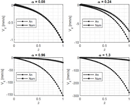
Figure 3: Effect of parameter α on the analytical and numerical predictions of velocityv_z (x ̃; y ̃=0,5), for WBF-1 [15] in a container of flat and parallel plates with two-dimensional domain. f=150 Hz, κ=∞.
Source: Own elaboration.

Figure 4: Effect of parameter α on the analytical and numerical predictions of the maximum velocity in v_z (x ̃; y ̃=0,5), for WBF-1 [15] in a container of flat and parallel plates with two-dimensional domain. f=150 Hz, κ=∞.
Source: Own elaboration.
IV. RESULTS ANALYSIS
Referring to figures 3 and 4, a permanent increase in the magnitude of the pseudo-analytical velocity profiles was observed. On the contrary, in numerical profiles, the magnitude of the velocity did not always increase as the intensity of the external magnetic field increased. In that sense, there were obvious differences between the results of each of the solution methodologies, as can also be seen in figure 5. Specifically, the container of figure 1 allowed to evaluate two aspects that had not been considered in previous studies [4]. First, the variation of the velocity in two dimensions was taken into account, that is, the height and width of the channel. Second, the joint effect of the tangential stresses at the ferrofluid-air interface, and the volumetric stresses within the same ferrofluid were evaluated. For this geometry, in figure 4 the saturation phenomenon of the profiles was again observed, for values of α≥1.
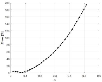
Figure 5: Effect of the parameter α on the percentage difference of the analytical and numerical predictions of the maximum velocity in , for WBF-1 [15] in a flat and parallel plate container with two-dimensional domain; , .
Source: Own elaboration.
V. PROPOSAL FOR IMPROVEMENT
In order to improve the accuracy of the responses obtained with the used models is necessary to adjust the model or their parameters. Accurate variables measurements can help to improve and prove these models.
VI. CONCLUSIONS
The model that describes the movement of ferrofluids by the action of an external rotating magnetic field, comprises a system of partial time-dependent differential equations describing the existing hydrodynamic, electrical and magnetic phenomena. This set of equations has a high complexity that currently prevents its analytical development. The literature reports some attempts to solve it but this has required the implementation of several approaches to obtain, thus, a pseudo-analytical solution, which in many cases departs from experimental reality. In this work the results obtained from this simplified analytical solution were compared with the numerical one. It was found that pseudo-analytical velocity profiles do not properly describe the phenomenon of saturation of ferrofluid. For this case, the magnitudes of the velocities were always increased, contrary to that obtained with the numerical profiles. Simulations were performed for parallel flat plate. In this way, we consider that the numerically generated velocity profiles, instead of the pseudo-analytical ones, are adequate to evaluate the performance of the ferro-hydrodynamic model.
VII. ACKNOWLEDGMENTS
The authors thank Universidad Industrial de Santander and Colciencias for its financial support (Grant 567). Furthermore, the first author would like to thank professors C. Rinaldi and A. Chaves for their selfless help.
VIII. REFERENCES
[1] R. Krauß, B. Reimann, R. Richter, I. Rehberg, M. Liu, “Fluid pumped by magnetic stress”, Applied Physics Letters, 2005, 86(2):024102.
[2] R. Krauß, M. Liu, B. Reimann, R. Richter, I. Rehberg, “Pumping fluid by magnetic surface stress”, New Journal of Physics, 2006, 8(1):18.
[3] A Chaves, “Magnetorheology in Rotating Magnetic Fields”, doctoral thesis, University of Puerto Rico Mayagüez Campus, 2007.
[4] A. Chaves-Guerrero, VA Peña-Cruz, C. Rinaldi, D. Fuentes-Díaz, “Spin-up flow in non-small magnetic fields: Numerical evaluation of the predictions of the common magnetization relaxation equations”, Physics of Fluids, 2017, 29(7):073102.
[5] Autor, “Evaluación del efecto de la ecuación de magnetización de Martsenyuk, Raikher y Shliomis sobre las predicciones de flujo de la teoría de difusión de momento angular interno”, doctoral thesis, Universidad Industrial de Santander, 2019.
[6] V. Zaitsev, M. Shliomis, “Entrainment of ferromagnetic suspension by a rotating field”, Journal of Applied Mechanics and Technical Physics, 1969, 10(5):696–700.
[7] O. Glazov, “Motion of a ferrosuspension in rotating magnetic fields”, Magnetohydrodynamics. 1975, 11(2):16–22.
[8] O. Glazov, “Role of higher harmonics in ferrosuspension motion in a rotating magnetic field”, Magnetohydrodynamics, 1975, 11(4):31.
[9] O. Glazov, “Velocity profiles for magnetic fluids in rotating magnetic fields”, Magnitnaya Gidrodynamika. 1982, 18:27.
[10] R. Rosensweig, J. Popplewell, R. Johnston, “Magnetic fluid motion in rotating field”, Journal of Magnetism and Magnetic Materials, 1990, 85(1):171–180.
[11] A. Chaves, M. Zahn, C. Rinaldi, “Spin-up flow of ferrofluids: Asymptotic theory and experimental measurements”, Physics of Fluids, 2008, 20(5):053102.23.
[12] A. Chaves, I. Torres-Diaz, C. Rinaldi, “Flow of ferrofluid in an annular gap in a rotating magnetic field”, Physics of Fluids, 2010, 22(9):092002.
[13] A. Chaves, C. Rinaldi, “Interfacial stress balances in structured continua and free surface flows in ferrofluids”, Physics of Fluids, 2014, 26(4):042101.
[14] A. Chaves, C. Rinaldi, S. Elborai, X. He, M. Zahn, “Bulk flow in ferrofluids in a uniform rotating magnetic field”, Physical Review Letters, 2006, 96(19):194501.
[15] I. Torres-Diaz, A. Cortes, Y. Cedeno-Mattei, O. Perales-Perez, C. Rinaldi, “Flows and torques in Brownian ferrofluids subjected to rotating uniform magnetic fields in a cylindrical and annular geometry”, Physics of Fluids, 2014, 26(1):012004.
[16] A. Chaves, F. Gutman, C. Rinaldi, “Torque and Bulk Flow of Ferrofluid in an Annular Gap Subjected to a Rotating Magnetic Field”, Transactions of the ASME, 2007, 129:412–422.
[17] C. Jimenez, H. Vargas, R. Correa, “Numerical Simulation of Ferromagnetic Fluid Flow in a Square Open Channel of Infinite Axial Length under the Effect of a Rotative Magnetic Field”, Indian Journal of Science and Technology, 2019, 11(48).
[18] V. Peña, A. Chaves, D. Fuentes. “Evaluación de dos ecuaciones de magnetización para la predicción del flujo de ferrofluido generado por un campo magnético rotando de alta amplitud”, undergraduate thesis, Universidad Industrial de Santander, Bucaramanga, 2015.
[19] W. Deen, Analysis of Transport Phenomena, Topics in Chemical Engineering vol. 3, New York, Oxford University Press, 1998.
[20] D. Condiff, JS. Dahler, “Fluid mechanical aspects of antisymmetric stress”, Physics of Fluids, 1964, 7(6):842–854.
[21] M. Shliomis, “Effective viscosity of magnetic suspensions”, Soviet Journal of Experimental and Theoretical Physics, 1972, 34:1291.
[22] M. Martsenyuk, “Viscosity of a suspension of ellipsoidal ferromagnetic particles in a magnetic field”, Journal of Applied Mechanics and Technical Physics, 1973, 14(5):664–669.
[23] M. Martsenyuk, Y. Raikher, M. Shliomis, “On the kinetics of magnetization of suspension of ferro-magnetic particles”, Journal of Experimental and Theoretical Physics, 1974, 38(2):413–416.
[24] V. Peña C., A. Chaves Guerrero, and D. Fuentes, “Análisis numérico para el fujo de un ferrofluido en el espacio anular entre dos cilindros concéntricos,” Rev. UIS Ing., vol. 11, no. 2, pp. 145–153, 2012.
![]()
In addition, Eq. (9) shows that the pair of efforts is continuous throughout the interface, considering that a and b represent the two phases that are part of the interface of the system under study. Therefore, the normal and tangential boundary conditions, for the internal angular momentum, are obtained through the internal product of Eq. (9) with the normal and tangential unit vectors, n and t. In this way, the following valid relationships are available for any point of the ferrofluid-air interface [13].
Likewise, the literature reports that with Eq. (13) and (14) the following relationships can be established for the solution of the system of hydrodynamic differential equations.
where T_nn and T_(nt )are the normal and tangential component of the stress tensor, respectively, which appear below.
In Eq. (13-16), ℏ represents the coefficient of curvature of the interface, ∇_s the surface gradient at the interface, γ the surface tension and K_s the surface current density. Additionally, in Eq. (13) it is taken into account that.
-
Equations describing the magnetic process
The system of magnetic equations has as one of its components the one related to the relaxation of magnetization. In the case where low amplitude rotary magnetic fields are applied, the magnetization equation of Shliomis [3,11,12,21] (Sh-72), Eq. (18) is used. Already for the case of flows in the presence of these fields but of high intensity, the magnetization equation of Martsenyuk, Raikher and Shliomis [22,23] (MRSh-74), Eq. (19) is used. It describes the behavior of the magnetization vector of the magnetic particle, in its attempt to align with the ERMF. In addition to these magnetic relaxation equations, the Maxwell equations, i.e., Ampère-Maxwell Law, Eq. (20), and Magnetic Field Gauss Law, Eq. (21), are used for the description of the rotating magnetic field present within the ferrofluid sample container.
where ε=(μ_0 χK^2 τ)/ζ=2/3 α^2 is called the perturbation parameter, [11]. The constants of the parallel and perpendicular relaxation times B_∥and B_⊥, respectively, appear below.
Similarly, to model the phenomenon of magnetic saturation of the ferrofluid, the Langevin equation, Eq. (23) will be used.
In this equation, subscripts 1 and 2 correspond to the components of the magnetic field intensity vector. The Langevin parameter, α, that appears in it is defined as,
That being said, to determine if a ferrofluid is subjected to a high or low amplitude magnetic field, the value of the said Langevin α parameter is taken as a reference. If α≪1 implies a low intensity magnetic field. On the contrary, a value of α≫1 implies one of high magnitude. In the first case (α≪1), there is a linear relationship between the equilibrium magnetization M_eq and the intensity of the magnetic field H. In the second case M_eq is approximately equal to the saturation magnetization of the ferrofluid. Similarly, to define the frequency of the external magnetic field, the dimensionless parameter Ω ̃ is examined. Thus, a value of Ω ̃≪1 describes a low frequency magnetic field and vice versa, values of Ω ̃≫1 correspond to high frequencies. In relation to the boundary conditions for the magnetic problem, these are condensed into two equations, the continuity of the normal component of the magnetic field density B, and that corresponding to the jump of the tangential component of the magnetic field intensity H, expressed as follows.
where K ̃_s is the current distribution on the surface of the walls of the ferrofluid container. The scalar components of the interfacial magnetic boundary equations are.
-
Geometry of flat and parallel plates
The physical system consists of a rectangular container of width and height δ, with walls on the lower surface and two sides (x ̃=0, y ̃=0 y y ̃=1) and infinite length (z direction), as can be seen in figure 1. It also contains a ferrofluid, which in its free surface comes into contact with the surrounding air (ferrofluid-air interface at x ̃=1). The rotating magnetic field is generated by two alternating current transport coils, out of phase 90^( ^° ) electric and 90^( ^° ) in space. The present fields are generated in the axial direction of the channel (magnetic field generated by the current in the xy plane and counterclockwise, (see figure 1). They also appear in the direction of the yz plane (magnetic field generated by the flow symbolized through circumferences, where the x inside the circumference constitutes the flow that enters the xy plane, and the filled circumferences, represent the flow that leaves the xy plane. (See figure 1). The origin of the coordinate axis it is located in the lower left corner of the front view of the channel. It is assumed that the resulting magnetic field rotates on the xz plane, because of the electric current flowing through each coil and its physical arrangement. Consequently, it is intended to predict profiles of: 1) the average linear velocity of the fluid in the axial direction v ̃=v ̃_z (x ̃,y ̃ ) i_z and 2) the angular velocity of the nanoparticles at the points of the xy plane of the channel, that is to say, ω ̃=ω ̃_x (x ̃,y ̃ ) i_x+ω ̃_y (x ̃,y ̃ ) i_y, considering that M ̃ ·∇ ̃H ̃=0, due to the assumption of uniformity of the rotating field. Finally, it is assumed that the physical arrangement of the external current sources makes it possible to define the intensity and the magnetic field density such as H ̃_z (t ̃ )=sin(t ̃ ) y B ̃_x (t ̃ )=cos(t ̃ ), respectively.
Figure 1: Diagram of the cross section of the rectangular channel and its associated variables for the application of IAMDT.
Source: Own elaboration.
III. METHODOLOGY OR PROCEDURES
-
Ferro-hydrodynamic equations, case α≪1
In order to obtain the solution to the system of differential equations of the hydrodynamic problem, a uniform ERMF was assumed, so that, M ̃ · ∇ ̃H ̃=0. Likewise, nullity was added in the divergence of the angular velocity of the nanoparticles, that is, ∇ ̃ ω ̃=0. Also, considering that there are no pressure differentials in the direction of the ferrofluid movement, you have to ∇ ̃p ̃=0. Finally, for the analytical solution the parameter η^'=0 was assumed, and therefore, κ→∞. Thus, the equations of hydrodynamic balance remain as:
By replacing Eq. (30) in Eq. (29), the nullity of the Laplacian of the linear velocity vector is obtained.
From Eq. (30) - (31) the linear velocity profiles are obtained, implementing the Fourier series (SF) method, for a channel of width W and height H. Resulting in Eq. (32) [5, 24].
- Ferro-hydrodynamic equations, case α≫1
For magnetic fields of intermediate or high intensity, the linear momentum balance equation remains the same, while the amount of IAM, bearing in mind Eq. (6), becomes.
Considering the coordinates in which IAM is presented (x and y coordinates), the respective component equations are (η^'≠0) [5].
Figure 2: Flowchart of methodology implemented in the development of the numerical algorithm, for the solution of the IAMDT ferrohydrodynamic problem.
Source: Own elaboration.
For their solution, these equations are discretized taking into account the presence of high intensity magnetic fields (α≫1) and the transmission of IAM (η^'≠0) [5]. In this order of ideas, the flow chart
corresponding to the methodology implemented for the numerical solution of the ferrohydrodynamic model is presented in Figure 2. First, the methodology initializes with the entry of the characteristic data of the ferrofluid sample. Next, the flow profiles are calculated, v ̃_z=f(x ̃,ω ̃_y ) y ω ̃_y=f(x ̃,v ̃_z,⟨ l ̃_y ⟩_t ), based on an average torque value, ⟨ l ̃_y ⟩_t, already determined. In the first iteration, the average torque values are initialized to zero. Subsequently, with these velocity values the magnetic problem is solved to calculate M ̃_x (x ̃,y ̃ ), M ̃_z (x ̃,y ̃ ), H ̃_x (x ̃,y ̃ ) y H ̃_z (x ̃,y ̃ ) and determine once again the value of the average torque, ⟨ l ̃_y ⟩_t^(k+1). This value is compared with that of the previous iteration, ⟨ l ̃_y ⟩_t^k, in order to establish convergence criteria. Once these are met, the values of the profiles found in the current iteration are printed, and set as the results of the algorithm.
- Comparison of velocity profiles
Then, in Figure 3 the effect of the approximations made in the analytical solution methodology is shown, in which ferrofluid saturation was not considered. It refers to the phenomenon in which the magnitude of the velocity is invariant as the intensity of the magnetic field increases, the magnetization vector of the ferrofluid nanoparticles remaining parallel to the direction of the external magnetic field. Similarly, the diffusion of IAM that occurs due to differences between the velocity of rotation of the nanoparticles and that of the carrier fluid was neglected. Although these approaches are necessary to solve the hydrodynamic equations in an analytical way, at the same time they restrict the validity of the model obtained for only ERMF values in which α≪1. In contrast, the velocity profiles obtained through the numerical solution algorithm are presented, in which such approaches are not required. In this figure, num and a represent the solutions obtained numerically and analytically using Fourier series, α= [0.08 0.24 0.96 1.3]. Now, to observe the differences in the flow predictions of each methodology, figure 4 shows the predicted maximum velocity values for each model, as a function of the value of α. The inability to predict the analytical solution is evident, due to the strong approximations that were made. Finally, figure 5 shows the error progression between the predictions of both models as the intensity of the rotating magnetic field increases.
Figure 3: Effect of parameter α on the analytical and numerical predictions of velocityv_z (x ̃; y ̃=0,5), for WBF-1 [15] in a container of flat and parallel plates with two-dimensional domain. f=150 Hz, κ=∞.
Source: Own elaboration.
Figure 4: Effect of parameter α on the analytical and numerical predictions of the maximum velocity in v_z (x ̃; y ̃=0,5), for WBF-1 [15] in a container of flat and parallel plates with two-dimensional domain. f=150 Hz, κ=∞.
Source: Own elaboration.
IV. RESULTS ANALYSIS
Referring to figures 3 and 4, a permanent increase in the magnitude of the pseudo-analytical velocity profiles was observed. On the contrary, in numerical profiles, the magnitude of the velocity did not always increase as the intensity of the external magnetic field increased. In that sense, there were obvious differences between the results of each of the solution methodologies, as can also be seen in figure 5. Specifically, the container of figure 1 allowed to evaluate two aspects that had not been considered in previous studies [4]. First, the variation of the velocity in two dimensions was taken into account, that is, the height and width of the channel. Second, the joint effect of the tangential stresses at the ferrofluid-air interface, and the volumetric stresses within the same ferrofluid were evaluated. For this geometry, in figure 4 the saturation phenomenon of the profiles was again observed, for values of α≥1.
Figure 5: Effect of the parameter α on the percentage difference of the analytical and numerical predictions of the maximum velocity in , for WBF-1 [15] in a flat and parallel plate container with two-dimensional domain; , .
Source: Own elaboration.
V. PROPOSAL FOR IMPROVEMENT
In order to improve the accuracy of the responses obtained with the used models is necessary to adjust the model or their parameters. Accurate variables measurements can help to improve and prove these models.
VI. CONCLUSIONS
The model that describes the movement of ferrofluids by the action of an external rotating magnetic field, comprises a system of partial time-dependent differential equations describing the existing hydrodynamic, electrical and magnetic phenomena. This set of equations has a high complexity that currently prevents its analytical development. The literature reports some attempts to solve it but this has required the implementation of several approaches to obtain, thus, a pseudo-analytical solution, which in many cases departs from experimental reality. In this work the results obtained from this simplified analytical solution were compared with the numerical one. It was found that pseudo-analytical velocity profiles do not properly describe the phenomenon of saturation of ferrofluid. For this case, the magnitudes of the velocities were always increased, contrary to that obtained with the numerical profiles. Simulations were performed for parallel flat plate. In this way, we consider that the numerically generated velocity profiles, instead of the pseudo-analytical ones, are adequate to evaluate the performance of the ferro-hydrodynamic model.
VII. ACKNOWLEDGMENTS
The authors thank Universidad Industrial de Santander and Colciencias for its financial support (Grant 567). Furthermore, the first author would like to thank professors C. Rinaldi and A. Chaves for their selfless help.
VIII. REFERENCES
[1] R. Krauß, B. Reimann, R. Richter, I. Rehberg, M. Liu, “Fluid pumped by magnetic stress”, Applied Physics Letters, 2005, 86(2):024102.
[2] R. Krauß, M. Liu, B. Reimann, R. Richter, I. Rehberg, “Pumping fluid by magnetic surface stress”, New Journal of Physics, 2006, 8(1):18.
[3] A Chaves, “Magnetorheology in Rotating Magnetic Fields”, doctoral thesis, University of Puerto Rico Mayagüez Campus, 2007.
[4] A. Chaves-Guerrero, VA Peña-Cruz, C. Rinaldi, D. Fuentes-Díaz, “Spin-up flow in non-small magnetic fields: Numerical evaluation of the predictions of the common magnetization relaxation equations”, Physics of Fluids, 2017, 29(7):073102.
[5] Autor, “Evaluación del efecto de la ecuación de magnetización de Martsenyuk, Raikher y Shliomis sobre las predicciones de flujo de la teoría de difusión de momento angular interno”, doctoral thesis, Universidad Industrial de Santander, 2019.
[6] V. Zaitsev, M. Shliomis, “Entrainment of ferromagnetic suspension by a rotating field”, Journal of Applied Mechanics and Technical Physics, 1969, 10(5):696–700.
[7] O. Glazov, “Motion of a ferrosuspension in rotating magnetic fields”, Magnetohydrodynamics. 1975, 11(2):16–22.
[8] O. Glazov, “Role of higher harmonics in ferrosuspension motion in a rotating magnetic field”, Magnetohydrodynamics, 1975, 11(4):31.
[9] O. Glazov, “Velocity profiles for magnetic fluids in rotating magnetic fields”, Magnitnaya Gidrodynamika. 1982, 18:27.
[10] R. Rosensweig, J. Popplewell, R. Johnston, “Magnetic fluid motion in rotating field”, Journal of Magnetism and Magnetic Materials, 1990, 85(1):171–180.
[11] A. Chaves, M. Zahn, C. Rinaldi, “Spin-up flow of ferrofluids: Asymptotic theory and experimental measurements”, Physics of Fluids, 2008, 20(5):053102.23.
[12] A. Chaves, I. Torres-Diaz, C. Rinaldi, “Flow of ferrofluid in an annular gap in a rotating magnetic field”, Physics of Fluids, 2010, 22(9):092002.
[13] A. Chaves, C. Rinaldi, “Interfacial stress balances in structured continua and free surface flows in ferrofluids”, Physics of Fluids, 2014, 26(4):042101.
[14] A. Chaves, C. Rinaldi, S. Elborai, X. He, M. Zahn, “Bulk flow in ferrofluids in a uniform rotating magnetic field”, Physical Review Letters, 2006, 96(19):194501.
[15] I. Torres-Diaz, A. Cortes, Y. Cedeno-Mattei, O. Perales-Perez, C. Rinaldi, “Flows and torques in Brownian ferrofluids subjected to rotating uniform magnetic fields in a cylindrical and annular geometry”, Physics of Fluids, 2014, 26(1):012004.
[16] A. Chaves, F. Gutman, C. Rinaldi, “Torque and Bulk Flow of Ferrofluid in an Annular Gap Subjected to a Rotating Magnetic Field”, Transactions of the ASME, 2007, 129:412–422.
[17] C. Jimenez, H. Vargas, R. Correa, “Numerical Simulation of Ferromagnetic Fluid Flow in a Square Open Channel of Infinite Axial Length under the Effect of a Rotative Magnetic Field”, Indian Journal of Science and Technology, 2019, 11(48).
[18] V. Peña, A. Chaves, D. Fuentes. “Evaluación de dos ecuaciones de magnetización para la predicción del flujo de ferrofluido generado por un campo magnético rotando de alta amplitud”, undergraduate thesis, Universidad Industrial de Santander, Bucaramanga, 2015.
[19] W. Deen, Analysis of Transport Phenomena, Topics in Chemical Engineering vol. 3, New York, Oxford University Press, 1998.
[20] D. Condiff, JS. Dahler, “Fluid mechanical aspects of antisymmetric stress”, Physics of Fluids, 1964, 7(6):842–854.
[21] M. Shliomis, “Effective viscosity of magnetic suspensions”, Soviet Journal of Experimental and Theoretical Physics, 1972, 34:1291.
[22] M. Martsenyuk, “Viscosity of a suspension of ellipsoidal ferromagnetic particles in a magnetic field”, Journal of Applied Mechanics and Technical Physics, 1973, 14(5):664–669.
[23] M. Martsenyuk, Y. Raikher, M. Shliomis, “On the kinetics of magnetization of suspension of ferro-magnetic particles”, Journal of Experimental and Theoretical Physics, 1974, 38(2):413–416.
[24] V. Peña C., A. Chaves Guerrero, and D. Fuentes, “Análisis numérico para el fujo de un ferrofluido en el espacio anular entre dos cilindros concéntricos,” Rev. UIS Ing., vol. 11, no. 2, pp. 145–153, 2012.
-
Equations describing the magnetic process
The system of magnetic equations has as one of its components the one related to the relaxation of magnetization. In the case where low amplitude rotary magnetic fields are applied, the magnetization equation of Shliomis [3,11,12,21] (Sh-72), Eq. (18) is used. Already for the case of flows in the presence of these fields but of high intensity, the magnetization equation of Martsenyuk, Raikher and Shliomis [22,23] (MRSh-74), Eq. (19) is used. It describes the behavior of the magnetization vector of the magnetic particle, in its attempt to align with the ERMF. In addition to these magnetic relaxation equations, the Maxwell equations, i.e., Ampère-Maxwell Law, Eq. (20), and Magnetic Field Gauss Law, Eq. (21), are used for the description of the rotating magnetic field present within the ferrofluid sample container.
where ε=(μ_0 χK^2 τ)/ζ=2/3 α^2 is called the perturbation parameter, [11]. The constants of the parallel and perpendicular relaxation times B_∥and B_⊥, respectively, appear below.
Similarly, to model the phenomenon of magnetic saturation of the ferrofluid, the Langevin equation, Eq. (23) will be used.
In this equation, subscripts 1 and 2 correspond to the components of the magnetic field intensity vector. The Langevin parameter, α, that appears in it is defined as,
That being said, to determine if a ferrofluid is subjected to a high or low amplitude magnetic field, the value of the said Langevin α parameter is taken as a reference. If α≪1 implies a low intensity magnetic field. On the contrary, a value of α≫1 implies one of high magnitude. In the first case (α≪1), there is a linear relationship between the equilibrium magnetization M_eq and the intensity of the magnetic field H. In the second case M_eq is approximately equal to the saturation magnetization of the ferrofluid. Similarly, to define the frequency of the external magnetic field, the dimensionless parameter Ω ̃ is examined. Thus, a value of Ω ̃≪1 describes a low frequency magnetic field and vice versa, values of Ω ̃≫1 correspond to high frequencies. In relation to the boundary conditions for the magnetic problem, these are condensed into two equations, the continuity of the normal component of the magnetic field density B, and that corresponding to the jump of the tangential component of the magnetic field intensity H, expressed as follows.
where K ̃_s is the current distribution on the surface of the walls of the ferrofluid container. The scalar components of the interfacial magnetic boundary equations are.
-
Geometry of flat and parallel plates
The physical system consists of a rectangular container of width and height δ, with walls on the lower surface and two sides (x ̃=0, y ̃=0 y y ̃=1) and infinite length (z direction), as can be seen in figure 1. It also contains a ferrofluid, which in its free surface comes into contact with the surrounding air (ferrofluid-air interface at x ̃=1). The rotating magnetic field is generated by two alternating current transport coils, out of phase 90^( ^° ) electric and 90^( ^° ) in space. The present fields are generated in the axial direction of the channel (magnetic field generated by the current in the xy plane and counterclockwise, (see figure 1). They also appear in the direction of the yz plane (magnetic field generated by the flow symbolized through circumferences, where the x inside the circumference constitutes the flow that enters the xy plane, and the filled circumferences, represent the flow that leaves the xy plane. (See figure 1). The origin of the coordinate axis it is located in the lower left corner of the front view of the channel. It is assumed that the resulting magnetic field rotates on the xz plane, because of the electric current flowing through each coil and its physical arrangement. Consequently, it is intended to predict profiles of: 1) the average linear velocity of the fluid in the axial direction v ̃=v ̃_z (x ̃,y ̃ ) i_z and 2) the angular velocity of the nanoparticles at the points of the xy plane of the channel, that is to say, ω ̃=ω ̃_x (x ̃,y ̃ ) i_x+ω ̃_y (x ̃,y ̃ ) i_y, considering that M ̃ ·∇ ̃H ̃=0, due to the assumption of uniformity of the rotating field. Finally, it is assumed that the physical arrangement of the external current sources makes it possible to define the intensity and the magnetic field density such as H ̃_z (t ̃ )=sin(t ̃ ) y B ̃_x (t ̃ )=cos(t ̃ ), respectively.
Figure 1: Diagram of the cross section of the rectangular channel and its associated variables for the application of IAMDT.
Source: Own elaboration.
III. METHODOLOGY OR PROCEDURES
-
Ferro-hydrodynamic equations, case α≪1
In order to obtain the solution to the system of differential equations of the hydrodynamic problem, a uniform ERMF was assumed, so that, M ̃ · ∇ ̃H ̃=0. Likewise, nullity was added in the divergence of the angular velocity of the nanoparticles, that is, ∇ ̃ ω ̃=0. Also, considering that there are no pressure differentials in the direction of the ferrofluid movement, you have to ∇ ̃p ̃=0. Finally, for the analytical solution the parameter η^'=0 was assumed, and therefore, κ→∞. Thus, the equations of hydrodynamic balance remain as:
By replacing Eq. (30) in Eq. (29), the nullity of the Laplacian of the linear velocity vector is obtained.
From Eq. (30) - (31) the linear velocity profiles are obtained, implementing the Fourier series (SF) method, for a channel of width W and height H. Resulting in Eq. (32) [5, 24].
- Ferro-hydrodynamic equations, case α≫1
For magnetic fields of intermediate or high intensity, the linear momentum balance equation remains the same, while the amount of IAM, bearing in mind Eq. (6), becomes.
Considering the coordinates in which IAM is presented (x and y coordinates), the respective component equations are (η^'≠0) [5].
Figure 2: Flowchart of methodology implemented in the development of the numerical algorithm, for the solution of the IAMDT ferrohydrodynamic problem.
Source: Own elaboration.
For their solution, these equations are discretized taking into account the presence of high intensity magnetic fields (α≫1) and the transmission of IAM (η^'≠0) [5]. In this order of ideas, the flow chart
corresponding to the methodology implemented for the numerical solution of the ferrohydrodynamic model is presented in Figure 2. First, the methodology initializes with the entry of the characteristic data of the ferrofluid sample. Next, the flow profiles are calculated, v ̃_z=f(x ̃,ω ̃_y ) y ω ̃_y=f(x ̃,v ̃_z,⟨ l ̃_y ⟩_t ), based on an average torque value, ⟨ l ̃_y ⟩_t, already determined. In the first iteration, the average torque values are initialized to zero. Subsequently, with these velocity values the magnetic problem is solved to calculate M ̃_x (x ̃,y ̃ ), M ̃_z (x ̃,y ̃ ), H ̃_x (x ̃,y ̃ ) y H ̃_z (x ̃,y ̃ ) and determine once again the value of the average torque, ⟨ l ̃_y ⟩_t^(k+1). This value is compared with that of the previous iteration, ⟨ l ̃_y ⟩_t^k, in order to establish convergence criteria. Once these are met, the values of the profiles found in the current iteration are printed, and set as the results of the algorithm.
- Comparison of velocity profiles
Then, in Figure 3 the effect of the approximations made in the analytical solution methodology is shown, in which ferrofluid saturation was not considered. It refers to the phenomenon in which the magnitude of the velocity is invariant as the intensity of the magnetic field increases, the magnetization vector of the ferrofluid nanoparticles remaining parallel to the direction of the external magnetic field. Similarly, the diffusion of IAM that occurs due to differences between the velocity of rotation of the nanoparticles and that of the carrier fluid was neglected. Although these approaches are necessary to solve the hydrodynamic equations in an analytical way, at the same time they restrict the validity of the model obtained for only ERMF values in which α≪1. In contrast, the velocity profiles obtained through the numerical solution algorithm are presented, in which such approaches are not required. In this figure, num and a represent the solutions obtained numerically and analytically using Fourier series, α= [0.08 0.24 0.96 1.3]. Now, to observe the differences in the flow predictions of each methodology, figure 4 shows the predicted maximum velocity values for each model, as a function of the value of α. The inability to predict the analytical solution is evident, due to the strong approximations that were made. Finally, figure 5 shows the error progression between the predictions of both models as the intensity of the rotating magnetic field increases.
Figure 3: Effect of parameter α on the analytical and numerical predictions of velocityv_z (x ̃; y ̃=0,5), for WBF-1 [15] in a container of flat and parallel plates with two-dimensional domain. f=150 Hz, κ=∞.
Source: Own elaboration.
Figure 4: Effect of parameter α on the analytical and numerical predictions of the maximum velocity in v_z (x ̃; y ̃=0,5), for WBF-1 [15] in a container of flat and parallel plates with two-dimensional domain. f=150 Hz, κ=∞.
Source: Own elaboration.
IV. RESULTS ANALYSIS
Referring to figures 3 and 4, a permanent increase in the magnitude of the pseudo-analytical velocity profiles was observed. On the contrary, in numerical profiles, the magnitude of the velocity did not always increase as the intensity of the external magnetic field increased. In that sense, there were obvious differences between the results of each of the solution methodologies, as can also be seen in figure 5. Specifically, the container of figure 1 allowed to evaluate two aspects that had not been considered in previous studies [4]. First, the variation of the velocity in two dimensions was taken into account, that is, the height and width of the channel. Second, the joint effect of the tangential stresses at the ferrofluid-air interface, and the volumetric stresses within the same ferrofluid were evaluated. For this geometry, in figure 4 the saturation phenomenon of the profiles was again observed, for values of α≥1.
Figure 5: Effect of the parameter α on the percentage difference of the analytical and numerical predictions of the maximum velocity in , for WBF-1 [15] in a flat and parallel plate container with two-dimensional domain; , .
Source: Own elaboration.
V. PROPOSAL FOR IMPROVEMENT
In order to improve the accuracy of the responses obtained with the used models is necessary to adjust the model or their parameters. Accurate variables measurements can help to improve and prove these models.
VI. CONCLUSIONS
The model that describes the movement of ferrofluids by the action of an external rotating magnetic field, comprises a system of partial time-dependent differential equations describing the existing hydrodynamic, electrical and magnetic phenomena. This set of equations has a high complexity that currently prevents its analytical development. The literature reports some attempts to solve it but this has required the implementation of several approaches to obtain, thus, a pseudo-analytical solution, which in many cases departs from experimental reality. In this work the results obtained from this simplified analytical solution were compared with the numerical one. It was found that pseudo-analytical velocity profiles do not properly describe the phenomenon of saturation of ferrofluid. For this case, the magnitudes of the velocities were always increased, contrary to that obtained with the numerical profiles. Simulations were performed for parallel flat plate. In this way, we consider that the numerically generated velocity profiles, instead of the pseudo-analytical ones, are adequate to evaluate the performance of the ferro-hydrodynamic model.
VII. ACKNOWLEDGMENTS
The authors thank Universidad Industrial de Santander and Colciencias for its financial support (Grant 567). Furthermore, the first author would like to thank professors C. Rinaldi and A. Chaves for their selfless help.
VIII. REFERENCES
[1] R. Krauß, B. Reimann, R. Richter, I. Rehberg, M. Liu, “Fluid pumped by magnetic stress”, Applied Physics Letters, 2005, 86(2):024102.
[2] R. Krauß, M. Liu, B. Reimann, R. Richter, I. Rehberg, “Pumping fluid by magnetic surface stress”, New Journal of Physics, 2006, 8(1):18.
[3] A Chaves, “Magnetorheology in Rotating Magnetic Fields”, doctoral thesis, University of Puerto Rico Mayagüez Campus, 2007.
[4] A. Chaves-Guerrero, VA Peña-Cruz, C. Rinaldi, D. Fuentes-Díaz, “Spin-up flow in non-small magnetic fields: Numerical evaluation of the predictions of the common magnetization relaxation equations”, Physics of Fluids, 2017, 29(7):073102.
[5] Autor, “Evaluación del efecto de la ecuación de magnetización de Martsenyuk, Raikher y Shliomis sobre las predicciones de flujo de la teoría de difusión de momento angular interno”, doctoral thesis, Universidad Industrial de Santander, 2019.
[6] V. Zaitsev, M. Shliomis, “Entrainment of ferromagnetic suspension by a rotating field”, Journal of Applied Mechanics and Technical Physics, 1969, 10(5):696–700.
[7] O. Glazov, “Motion of a ferrosuspension in rotating magnetic fields”, Magnetohydrodynamics. 1975, 11(2):16–22.
[8] O. Glazov, “Role of higher harmonics in ferrosuspension motion in a rotating magnetic field”, Magnetohydrodynamics, 1975, 11(4):31.
[9] O. Glazov, “Velocity profiles for magnetic fluids in rotating magnetic fields”, Magnitnaya Gidrodynamika. 1982, 18:27.
[10] R. Rosensweig, J. Popplewell, R. Johnston, “Magnetic fluid motion in rotating field”, Journal of Magnetism and Magnetic Materials, 1990, 85(1):171–180.
[11] A. Chaves, M. Zahn, C. Rinaldi, “Spin-up flow of ferrofluids: Asymptotic theory and experimental measurements”, Physics of Fluids, 2008, 20(5):053102.23.
[12] A. Chaves, I. Torres-Diaz, C. Rinaldi, “Flow of ferrofluid in an annular gap in a rotating magnetic field”, Physics of Fluids, 2010, 22(9):092002.
[13] A. Chaves, C. Rinaldi, “Interfacial stress balances in structured continua and free surface flows in ferrofluids”, Physics of Fluids, 2014, 26(4):042101.
[14] A. Chaves, C. Rinaldi, S. Elborai, X. He, M. Zahn, “Bulk flow in ferrofluids in a uniform rotating magnetic field”, Physical Review Letters, 2006, 96(19):194501.
[15] I. Torres-Diaz, A. Cortes, Y. Cedeno-Mattei, O. Perales-Perez, C. Rinaldi, “Flows and torques in Brownian ferrofluids subjected to rotating uniform magnetic fields in a cylindrical and annular geometry”, Physics of Fluids, 2014, 26(1):012004.
[16] A. Chaves, F. Gutman, C. Rinaldi, “Torque and Bulk Flow of Ferrofluid in an Annular Gap Subjected to a Rotating Magnetic Field”, Transactions of the ASME, 2007, 129:412–422.
[17] C. Jimenez, H. Vargas, R. Correa, “Numerical Simulation of Ferromagnetic Fluid Flow in a Square Open Channel of Infinite Axial Length under the Effect of a Rotative Magnetic Field”, Indian Journal of Science and Technology, 2019, 11(48).
[18] V. Peña, A. Chaves, D. Fuentes. “Evaluación de dos ecuaciones de magnetización para la predicción del flujo de ferrofluido generado por un campo magnético rotando de alta amplitud”, undergraduate thesis, Universidad Industrial de Santander, Bucaramanga, 2015.
[19] W. Deen, Analysis of Transport Phenomena, Topics in Chemical Engineering vol. 3, New York, Oxford University Press, 1998.
[20] D. Condiff, JS. Dahler, “Fluid mechanical aspects of antisymmetric stress”, Physics of Fluids, 1964, 7(6):842–854.
[21] M. Shliomis, “Effective viscosity of magnetic suspensions”, Soviet Journal of Experimental and Theoretical Physics, 1972, 34:1291.
[22] M. Martsenyuk, “Viscosity of a suspension of ellipsoidal ferromagnetic particles in a magnetic field”, Journal of Applied Mechanics and Technical Physics, 1973, 14(5):664–669.
[23] M. Martsenyuk, Y. Raikher, M. Shliomis, “On the kinetics of magnetization of suspension of ferro-magnetic particles”, Journal of Experimental and Theoretical Physics, 1974, 38(2):413–416.
[24] V. Peña C., A. Chaves Guerrero, and D. Fuentes, “Análisis numérico para el fujo de un ferrofluido en el espacio anular entre dos cilindros concéntricos,” Rev. UIS Ing., vol. 11, no. 2, pp. 145–153, 2012.
![]()
In this equation, subscripts 1 and 2 correspond to the components of the magnetic field intensity vector. The Langevin parameter, α, that appears in it is defined as,
That being said, to determine if a ferrofluid is subjected to a high or low amplitude magnetic field, the value of the said Langevin α parameter is taken as a reference. If α≪1 implies a low intensity magnetic field. On the contrary, a value of α≫1 implies one of high magnitude. In the first case (α≪1), there is a linear relationship between the equilibrium magnetization M_eq and the intensity of the magnetic field H. In the second case M_eq is approximately equal to the saturation magnetization of the ferrofluid. Similarly, to define the frequency of the external magnetic field, the dimensionless parameter Ω ̃ is examined. Thus, a value of Ω ̃≪1 describes a low frequency magnetic field and vice versa, values of Ω ̃≫1 correspond to high frequencies. In relation to the boundary conditions for the magnetic problem, these are condensed into two equations, the continuity of the normal component of the magnetic field density B, and that corresponding to the jump of the tangential component of the magnetic field intensity H, expressed as follows.
where K ̃_s is the current distribution on the surface of the walls of the ferrofluid container. The scalar components of the interfacial magnetic boundary equations are.
-
Geometry of flat and parallel plates
The physical system consists of a rectangular container of width and height δ, with walls on the lower surface and two sides (x ̃=0, y ̃=0 y y ̃=1) and infinite length (z direction), as can be seen in figure 1. It also contains a ferrofluid, which in its free surface comes into contact with the surrounding air (ferrofluid-air interface at x ̃=1). The rotating magnetic field is generated by two alternating current transport coils, out of phase 90^( ^° ) electric and 90^( ^° ) in space. The present fields are generated in the axial direction of the channel (magnetic field generated by the current in the xy plane and counterclockwise, (see figure 1). They also appear in the direction of the yz plane (magnetic field generated by the flow symbolized through circumferences, where the x inside the circumference constitutes the flow that enters the xy plane, and the filled circumferences, represent the flow that leaves the xy plane. (See figure 1). The origin of the coordinate axis it is located in the lower left corner of the front view of the channel. It is assumed that the resulting magnetic field rotates on the xz plane, because of the electric current flowing through each coil and its physical arrangement. Consequently, it is intended to predict profiles of: 1) the average linear velocity of the fluid in the axial direction v ̃=v ̃_z (x ̃,y ̃ ) i_z and 2) the angular velocity of the nanoparticles at the points of the xy plane of the channel, that is to say, ω ̃=ω ̃_x (x ̃,y ̃ ) i_x+ω ̃_y (x ̃,y ̃ ) i_y, considering that M ̃ ·∇ ̃H ̃=0, due to the assumption of uniformity of the rotating field. Finally, it is assumed that the physical arrangement of the external current sources makes it possible to define the intensity and the magnetic field density such as H ̃_z (t ̃ )=sin(t ̃ ) y B ̃_x (t ̃ )=cos(t ̃ ), respectively.
Figure 1: Diagram of the cross section of the rectangular channel and its associated variables for the application of IAMDT.
Source: Own elaboration.
III. METHODOLOGY OR PROCEDURES
-
Ferro-hydrodynamic equations, case α≪1
In order to obtain the solution to the system of differential equations of the hydrodynamic problem, a uniform ERMF was assumed, so that, M ̃ · ∇ ̃H ̃=0. Likewise, nullity was added in the divergence of the angular velocity of the nanoparticles, that is, ∇ ̃ ω ̃=0. Also, considering that there are no pressure differentials in the direction of the ferrofluid movement, you have to ∇ ̃p ̃=0. Finally, for the analytical solution the parameter η^'=0 was assumed, and therefore, κ→∞. Thus, the equations of hydrodynamic balance remain as:
By replacing Eq. (30) in Eq. (29), the nullity of the Laplacian of the linear velocity vector is obtained.
From Eq. (30) - (31) the linear velocity profiles are obtained, implementing the Fourier series (SF) method, for a channel of width W and height H. Resulting in Eq. (32) [5, 24].
- Ferro-hydrodynamic equations, case α≫1
For magnetic fields of intermediate or high intensity, the linear momentum balance equation remains the same, while the amount of IAM, bearing in mind Eq. (6), becomes.
Considering the coordinates in which IAM is presented (x and y coordinates), the respective component equations are (η^'≠0) [5].
Figure 2: Flowchart of methodology implemented in the development of the numerical algorithm, for the solution of the IAMDT ferrohydrodynamic problem.
Source: Own elaboration.
For their solution, these equations are discretized taking into account the presence of high intensity magnetic fields (α≫1) and the transmission of IAM (η^'≠0) [5]. In this order of ideas, the flow chart
corresponding to the methodology implemented for the numerical solution of the ferrohydrodynamic model is presented in Figure 2. First, the methodology initializes with the entry of the characteristic data of the ferrofluid sample. Next, the flow profiles are calculated, v ̃_z=f(x ̃,ω ̃_y ) y ω ̃_y=f(x ̃,v ̃_z,⟨ l ̃_y ⟩_t ), based on an average torque value, ⟨ l ̃_y ⟩_t, already determined. In the first iteration, the average torque values are initialized to zero. Subsequently, with these velocity values the magnetic problem is solved to calculate M ̃_x (x ̃,y ̃ ), M ̃_z (x ̃,y ̃ ), H ̃_x (x ̃,y ̃ ) y H ̃_z (x ̃,y ̃ ) and determine once again the value of the average torque, ⟨ l ̃_y ⟩_t^(k+1). This value is compared with that of the previous iteration, ⟨ l ̃_y ⟩_t^k, in order to establish convergence criteria. Once these are met, the values of the profiles found in the current iteration are printed, and set as the results of the algorithm.
- Comparison of velocity profiles
Then, in Figure 3 the effect of the approximations made in the analytical solution methodology is shown, in which ferrofluid saturation was not considered. It refers to the phenomenon in which the magnitude of the velocity is invariant as the intensity of the magnetic field increases, the magnetization vector of the ferrofluid nanoparticles remaining parallel to the direction of the external magnetic field. Similarly, the diffusion of IAM that occurs due to differences between the velocity of rotation of the nanoparticles and that of the carrier fluid was neglected. Although these approaches are necessary to solve the hydrodynamic equations in an analytical way, at the same time they restrict the validity of the model obtained for only ERMF values in which α≪1. In contrast, the velocity profiles obtained through the numerical solution algorithm are presented, in which such approaches are not required. In this figure, num and a represent the solutions obtained numerically and analytically using Fourier series, α= [0.08 0.24 0.96 1.3]. Now, to observe the differences in the flow predictions of each methodology, figure 4 shows the predicted maximum velocity values for each model, as a function of the value of α. The inability to predict the analytical solution is evident, due to the strong approximations that were made. Finally, figure 5 shows the error progression between the predictions of both models as the intensity of the rotating magnetic field increases.
Figure 3: Effect of parameter α on the analytical and numerical predictions of velocityv_z (x ̃; y ̃=0,5), for WBF-1 [15] in a container of flat and parallel plates with two-dimensional domain. f=150 Hz, κ=∞.
Source: Own elaboration.
Figure 4: Effect of parameter α on the analytical and numerical predictions of the maximum velocity in v_z (x ̃; y ̃=0,5), for WBF-1 [15] in a container of flat and parallel plates with two-dimensional domain. f=150 Hz, κ=∞.
Source: Own elaboration.
IV. RESULTS ANALYSIS
Referring to figures 3 and 4, a permanent increase in the magnitude of the pseudo-analytical velocity profiles was observed. On the contrary, in numerical profiles, the magnitude of the velocity did not always increase as the intensity of the external magnetic field increased. In that sense, there were obvious differences between the results of each of the solution methodologies, as can also be seen in figure 5. Specifically, the container of figure 1 allowed to evaluate two aspects that had not been considered in previous studies [4]. First, the variation of the velocity in two dimensions was taken into account, that is, the height and width of the channel. Second, the joint effect of the tangential stresses at the ferrofluid-air interface, and the volumetric stresses within the same ferrofluid were evaluated. For this geometry, in figure 4 the saturation phenomenon of the profiles was again observed, for values of α≥1.
Figure 5: Effect of the parameter α on the percentage difference of the analytical and numerical predictions of the maximum velocity in , for WBF-1 [15] in a flat and parallel plate container with two-dimensional domain; , .
Source: Own elaboration.
V. PROPOSAL FOR IMPROVEMENT
In order to improve the accuracy of the responses obtained with the used models is necessary to adjust the model or their parameters. Accurate variables measurements can help to improve and prove these models.
VI. CONCLUSIONS
The model that describes the movement of ferrofluids by the action of an external rotating magnetic field, comprises a system of partial time-dependent differential equations describing the existing hydrodynamic, electrical and magnetic phenomena. This set of equations has a high complexity that currently prevents its analytical development. The literature reports some attempts to solve it but this has required the implementation of several approaches to obtain, thus, a pseudo-analytical solution, which in many cases departs from experimental reality. In this work the results obtained from this simplified analytical solution were compared with the numerical one. It was found that pseudo-analytical velocity profiles do not properly describe the phenomenon of saturation of ferrofluid. For this case, the magnitudes of the velocities were always increased, contrary to that obtained with the numerical profiles. Simulations were performed for parallel flat plate. In this way, we consider that the numerically generated velocity profiles, instead of the pseudo-analytical ones, are adequate to evaluate the performance of the ferro-hydrodynamic model.
VII. ACKNOWLEDGMENTS
The authors thank Universidad Industrial de Santander and Colciencias for its financial support (Grant 567). Furthermore, the first author would like to thank professors C. Rinaldi and A. Chaves for their selfless help.
VIII. REFERENCES
[1] R. Krauß, B. Reimann, R. Richter, I. Rehberg, M. Liu, “Fluid pumped by magnetic stress”, Applied Physics Letters, 2005, 86(2):024102.
[2] R. Krauß, M. Liu, B. Reimann, R. Richter, I. Rehberg, “Pumping fluid by magnetic surface stress”, New Journal of Physics, 2006, 8(1):18.
[3] A Chaves, “Magnetorheology in Rotating Magnetic Fields”, doctoral thesis, University of Puerto Rico Mayagüez Campus, 2007.
[4] A. Chaves-Guerrero, VA Peña-Cruz, C. Rinaldi, D. Fuentes-Díaz, “Spin-up flow in non-small magnetic fields: Numerical evaluation of the predictions of the common magnetization relaxation equations”, Physics of Fluids, 2017, 29(7):073102.
[5] Autor, “Evaluación del efecto de la ecuación de magnetización de Martsenyuk, Raikher y Shliomis sobre las predicciones de flujo de la teoría de difusión de momento angular interno”, doctoral thesis, Universidad Industrial de Santander, 2019.
[6] V. Zaitsev, M. Shliomis, “Entrainment of ferromagnetic suspension by a rotating field”, Journal of Applied Mechanics and Technical Physics, 1969, 10(5):696–700.
[7] O. Glazov, “Motion of a ferrosuspension in rotating magnetic fields”, Magnetohydrodynamics. 1975, 11(2):16–22.
[8] O. Glazov, “Role of higher harmonics in ferrosuspension motion in a rotating magnetic field”, Magnetohydrodynamics, 1975, 11(4):31.
[9] O. Glazov, “Velocity profiles for magnetic fluids in rotating magnetic fields”, Magnitnaya Gidrodynamika. 1982, 18:27.
[10] R. Rosensweig, J. Popplewell, R. Johnston, “Magnetic fluid motion in rotating field”, Journal of Magnetism and Magnetic Materials, 1990, 85(1):171–180.
[11] A. Chaves, M. Zahn, C. Rinaldi, “Spin-up flow of ferrofluids: Asymptotic theory and experimental measurements”, Physics of Fluids, 2008, 20(5):053102.23.
[12] A. Chaves, I. Torres-Diaz, C. Rinaldi, “Flow of ferrofluid in an annular gap in a rotating magnetic field”, Physics of Fluids, 2010, 22(9):092002.
[13] A. Chaves, C. Rinaldi, “Interfacial stress balances in structured continua and free surface flows in ferrofluids”, Physics of Fluids, 2014, 26(4):042101.
[14] A. Chaves, C. Rinaldi, S. Elborai, X. He, M. Zahn, “Bulk flow in ferrofluids in a uniform rotating magnetic field”, Physical Review Letters, 2006, 96(19):194501.
[15] I. Torres-Diaz, A. Cortes, Y. Cedeno-Mattei, O. Perales-Perez, C. Rinaldi, “Flows and torques in Brownian ferrofluids subjected to rotating uniform magnetic fields in a cylindrical and annular geometry”, Physics of Fluids, 2014, 26(1):012004.
[16] A. Chaves, F. Gutman, C. Rinaldi, “Torque and Bulk Flow of Ferrofluid in an Annular Gap Subjected to a Rotating Magnetic Field”, Transactions of the ASME, 2007, 129:412–422.
[17] C. Jimenez, H. Vargas, R. Correa, “Numerical Simulation of Ferromagnetic Fluid Flow in a Square Open Channel of Infinite Axial Length under the Effect of a Rotative Magnetic Field”, Indian Journal of Science and Technology, 2019, 11(48).
[18] V. Peña, A. Chaves, D. Fuentes. “Evaluación de dos ecuaciones de magnetización para la predicción del flujo de ferrofluido generado por un campo magnético rotando de alta amplitud”, undergraduate thesis, Universidad Industrial de Santander, Bucaramanga, 2015.
[19] W. Deen, Analysis of Transport Phenomena, Topics in Chemical Engineering vol. 3, New York, Oxford University Press, 1998.
[20] D. Condiff, JS. Dahler, “Fluid mechanical aspects of antisymmetric stress”, Physics of Fluids, 1964, 7(6):842–854.
[21] M. Shliomis, “Effective viscosity of magnetic suspensions”, Soviet Journal of Experimental and Theoretical Physics, 1972, 34:1291.
[22] M. Martsenyuk, “Viscosity of a suspension of ellipsoidal ferromagnetic particles in a magnetic field”, Journal of Applied Mechanics and Technical Physics, 1973, 14(5):664–669.
[23] M. Martsenyuk, Y. Raikher, M. Shliomis, “On the kinetics of magnetization of suspension of ferro-magnetic particles”, Journal of Experimental and Theoretical Physics, 1974, 38(2):413–416.
[24] V. Peña C., A. Chaves Guerrero, and D. Fuentes, “Análisis numérico para el fujo de un ferrofluido en el espacio anular entre dos cilindros concéntricos,” Rev. UIS Ing., vol. 11, no. 2, pp. 145–153, 2012.
-
Geometry of flat and parallel plates
The physical system consists of a rectangular container of width and height δ, with walls on the lower surface and two sides (x ̃=0, y ̃=0 y y ̃=1) and infinite length (z direction), as can be seen in figure 1. It also contains a ferrofluid, which in its free surface comes into contact with the surrounding air (ferrofluid-air interface at x ̃=1). The rotating magnetic field is generated by two alternating current transport coils, out of phase 90^( ^° ) electric and 90^( ^° ) in space. The present fields are generated in the axial direction of the channel (magnetic field generated by the current in the xy plane and counterclockwise, (see figure 1). They also appear in the direction of the yz plane (magnetic field generated by the flow symbolized through circumferences, where the x inside the circumference constitutes the flow that enters the xy plane, and the filled circumferences, represent the flow that leaves the xy plane. (See figure 1). The origin of the coordinate axis it is located in the lower left corner of the front view of the channel. It is assumed that the resulting magnetic field rotates on the xz plane, because of the electric current flowing through each coil and its physical arrangement. Consequently, it is intended to predict profiles of: 1) the average linear velocity of the fluid in the axial direction v ̃=v ̃_z (x ̃,y ̃ ) i_z and 2) the angular velocity of the nanoparticles at the points of the xy plane of the channel, that is to say, ω ̃=ω ̃_x (x ̃,y ̃ ) i_x+ω ̃_y (x ̃,y ̃ ) i_y, considering that M ̃ ·∇ ̃H ̃=0, due to the assumption of uniformity of the rotating field. Finally, it is assumed that the physical arrangement of the external current sources makes it possible to define the intensity and the magnetic field density such as H ̃_z (t ̃ )=sin(t ̃ ) y B ̃_x (t ̃ )=cos(t ̃ ), respectively.
Figure 1: Diagram of the cross section of the rectangular channel and its associated variables for the application of IAMDT.
Source: Own elaboration.
-
Ferro-hydrodynamic equations, case α≪1
In order to obtain the solution to the system of differential equations of the hydrodynamic problem, a uniform ERMF was assumed, so that, M ̃ · ∇ ̃H ̃=0. Likewise, nullity was added in the divergence of the angular velocity of the nanoparticles, that is, ∇ ̃ ω ̃=0. Also, considering that there are no pressure differentials in the direction of the ferrofluid movement, you have to ∇ ̃p ̃=0. Finally, for the analytical solution the parameter η^'=0 was assumed, and therefore, κ→∞. Thus, the equations of hydrodynamic balance remain as:
By replacing Eq. (30) in Eq. (29), the nullity of the Laplacian of the linear velocity vector is obtained.
From Eq. (30) - (31) the linear velocity profiles are obtained, implementing the Fourier series (SF) method, for a channel of width W and height H. Resulting in Eq. (32) [5, 24].
- Ferro-hydrodynamic equations, case α≫1
For magnetic fields of intermediate or high intensity, the linear momentum balance equation remains the same, while the amount of IAM, bearing in mind Eq. (6), becomes.
Considering the coordinates in which IAM is presented (x and y coordinates), the respective component equations are (η^'≠0) [5].
Figure 2: Flowchart of methodology implemented in the development of the numerical algorithm, for the solution of the IAMDT ferrohydrodynamic problem.
Source: Own elaboration.
For their solution, these equations are discretized taking into account the presence of high intensity magnetic fields (α≫1) and the transmission of IAM (η^'≠0) [5]. In this order of ideas, the flow chart
corresponding to the methodology implemented for the numerical solution of the ferrohydrodynamic model is presented in Figure 2. First, the methodology initializes with the entry of the characteristic data of the ferrofluid sample. Next, the flow profiles are calculated, v ̃_z=f(x ̃,ω ̃_y ) y ω ̃_y=f(x ̃,v ̃_z,⟨ l ̃_y ⟩_t ), based on an average torque value, ⟨ l ̃_y ⟩_t, already determined. In the first iteration, the average torque values are initialized to zero. Subsequently, with these velocity values the magnetic problem is solved to calculate M ̃_x (x ̃,y ̃ ), M ̃_z (x ̃,y ̃ ), H ̃_x (x ̃,y ̃ ) y H ̃_z (x ̃,y ̃ ) and determine once again the value of the average torque, ⟨ l ̃_y ⟩_t^(k+1). This value is compared with that of the previous iteration, ⟨ l ̃_y ⟩_t^k, in order to establish convergence criteria. Once these are met, the values of the profiles found in the current iteration are printed, and set as the results of the algorithm.
- Comparison of velocity profiles
Then, in Figure 3 the effect of the approximations made in the analytical solution methodology is shown, in which ferrofluid saturation was not considered. It refers to the phenomenon in which the magnitude of the velocity is invariant as the intensity of the magnetic field increases, the magnetization vector of the ferrofluid nanoparticles remaining parallel to the direction of the external magnetic field. Similarly, the diffusion of IAM that occurs due to differences between the velocity of rotation of the nanoparticles and that of the carrier fluid was neglected. Although these approaches are necessary to solve the hydrodynamic equations in an analytical way, at the same time they restrict the validity of the model obtained for only ERMF values in which α≪1. In contrast, the velocity profiles obtained through the numerical solution algorithm are presented, in which such approaches are not required. In this figure, num and a represent the solutions obtained numerically and analytically using Fourier series, α= [0.08 0.24 0.96 1.3]. Now, to observe the differences in the flow predictions of each methodology, figure 4 shows the predicted maximum velocity values for each model, as a function of the value of α. The inability to predict the analytical solution is evident, due to the strong approximations that were made. Finally, figure 5 shows the error progression between the predictions of both models as the intensity of the rotating magnetic field increases.
Figure 3: Effect of parameter α on the analytical and numerical predictions of velocityv_z (x ̃; y ̃=0,5), for WBF-1 [15] in a container of flat and parallel plates with two-dimensional domain. f=150 Hz, κ=∞.
Source: Own elaboration.
Figure 4: Effect of parameter α on the analytical and numerical predictions of the maximum velocity in v_z (x ̃; y ̃=0,5), for WBF-1 [15] in a container of flat and parallel plates with two-dimensional domain. f=150 Hz, κ=∞.
Source: Own elaboration.
IV. RESULTS ANALYSIS
Referring to figures 3 and 4, a permanent increase in the magnitude of the pseudo-analytical velocity profiles was observed. On the contrary, in numerical profiles, the magnitude of the velocity did not always increase as the intensity of the external magnetic field increased. In that sense, there were obvious differences between the results of each of the solution methodologies, as can also be seen in figure 5. Specifically, the container of figure 1 allowed to evaluate two aspects that had not been considered in previous studies [4]. First, the variation of the velocity in two dimensions was taken into account, that is, the height and width of the channel. Second, the joint effect of the tangential stresses at the ferrofluid-air interface, and the volumetric stresses within the same ferrofluid were evaluated. For this geometry, in figure 4 the saturation phenomenon of the profiles was again observed, for values of α≥1.
Figure 5: Effect of the parameter α on the percentage difference of the analytical and numerical predictions of the maximum velocity in , for WBF-1 [15] in a flat and parallel plate container with two-dimensional domain; , .
Source: Own elaboration.
V. PROPOSAL FOR IMPROVEMENT
In order to improve the accuracy of the responses obtained with the used models is necessary to adjust the model or their parameters. Accurate variables measurements can help to improve and prove these models.
VI. CONCLUSIONS
The model that describes the movement of ferrofluids by the action of an external rotating magnetic field, comprises a system of partial time-dependent differential equations describing the existing hydrodynamic, electrical and magnetic phenomena. This set of equations has a high complexity that currently prevents its analytical development. The literature reports some attempts to solve it but this has required the implementation of several approaches to obtain, thus, a pseudo-analytical solution, which in many cases departs from experimental reality. In this work the results obtained from this simplified analytical solution were compared with the numerical one. It was found that pseudo-analytical velocity profiles do not properly describe the phenomenon of saturation of ferrofluid. For this case, the magnitudes of the velocities were always increased, contrary to that obtained with the numerical profiles. Simulations were performed for parallel flat plate. In this way, we consider that the numerically generated velocity profiles, instead of the pseudo-analytical ones, are adequate to evaluate the performance of the ferro-hydrodynamic model.
VII. ACKNOWLEDGMENTS
The authors thank Universidad Industrial de Santander and Colciencias for its financial support (Grant 567). Furthermore, the first author would like to thank professors C. Rinaldi and A. Chaves for their selfless help.
VIII. REFERENCES
[1] R. Krauß, B. Reimann, R. Richter, I. Rehberg, M. Liu, “Fluid pumped by magnetic stress”, Applied Physics Letters, 2005, 86(2):024102.
[2] R. Krauß, M. Liu, B. Reimann, R. Richter, I. Rehberg, “Pumping fluid by magnetic surface stress”, New Journal of Physics, 2006, 8(1):18.
[3] A Chaves, “Magnetorheology in Rotating Magnetic Fields”, doctoral thesis, University of Puerto Rico Mayagüez Campus, 2007.
[4] A. Chaves-Guerrero, VA Peña-Cruz, C. Rinaldi, D. Fuentes-Díaz, “Spin-up flow in non-small magnetic fields: Numerical evaluation of the predictions of the common magnetization relaxation equations”, Physics of Fluids, 2017, 29(7):073102.
[5] Autor, “Evaluación del efecto de la ecuación de magnetización de Martsenyuk, Raikher y Shliomis sobre las predicciones de flujo de la teoría de difusión de momento angular interno”, doctoral thesis, Universidad Industrial de Santander, 2019.
[6] V. Zaitsev, M. Shliomis, “Entrainment of ferromagnetic suspension by a rotating field”, Journal of Applied Mechanics and Technical Physics, 1969, 10(5):696–700.
[7] O. Glazov, “Motion of a ferrosuspension in rotating magnetic fields”, Magnetohydrodynamics. 1975, 11(2):16–22.
[8] O. Glazov, “Role of higher harmonics in ferrosuspension motion in a rotating magnetic field”, Magnetohydrodynamics, 1975, 11(4):31.
[9] O. Glazov, “Velocity profiles for magnetic fluids in rotating magnetic fields”, Magnitnaya Gidrodynamika. 1982, 18:27.
[10] R. Rosensweig, J. Popplewell, R. Johnston, “Magnetic fluid motion in rotating field”, Journal of Magnetism and Magnetic Materials, 1990, 85(1):171–180.
[11] A. Chaves, M. Zahn, C. Rinaldi, “Spin-up flow of ferrofluids: Asymptotic theory and experimental measurements”, Physics of Fluids, 2008, 20(5):053102.23.
[12] A. Chaves, I. Torres-Diaz, C. Rinaldi, “Flow of ferrofluid in an annular gap in a rotating magnetic field”, Physics of Fluids, 2010, 22(9):092002.
[13] A. Chaves, C. Rinaldi, “Interfacial stress balances in structured continua and free surface flows in ferrofluids”, Physics of Fluids, 2014, 26(4):042101.
[14] A. Chaves, C. Rinaldi, S. Elborai, X. He, M. Zahn, “Bulk flow in ferrofluids in a uniform rotating magnetic field”, Physical Review Letters, 2006, 96(19):194501.
[15] I. Torres-Diaz, A. Cortes, Y. Cedeno-Mattei, O. Perales-Perez, C. Rinaldi, “Flows and torques in Brownian ferrofluids subjected to rotating uniform magnetic fields in a cylindrical and annular geometry”, Physics of Fluids, 2014, 26(1):012004.
[16] A. Chaves, F. Gutman, C. Rinaldi, “Torque and Bulk Flow of Ferrofluid in an Annular Gap Subjected to a Rotating Magnetic Field”, Transactions of the ASME, 2007, 129:412–422.
[17] C. Jimenez, H. Vargas, R. Correa, “Numerical Simulation of Ferromagnetic Fluid Flow in a Square Open Channel of Infinite Axial Length under the Effect of a Rotative Magnetic Field”, Indian Journal of Science and Technology, 2019, 11(48).
[18] V. Peña, A. Chaves, D. Fuentes. “Evaluación de dos ecuaciones de magnetización para la predicción del flujo de ferrofluido generado por un campo magnético rotando de alta amplitud”, undergraduate thesis, Universidad Industrial de Santander, Bucaramanga, 2015.
[19] W. Deen, Analysis of Transport Phenomena, Topics in Chemical Engineering vol. 3, New York, Oxford University Press, 1998.
[20] D. Condiff, JS. Dahler, “Fluid mechanical aspects of antisymmetric stress”, Physics of Fluids, 1964, 7(6):842–854.
[21] M. Shliomis, “Effective viscosity of magnetic suspensions”, Soviet Journal of Experimental and Theoretical Physics, 1972, 34:1291.
[22] M. Martsenyuk, “Viscosity of a suspension of ellipsoidal ferromagnetic particles in a magnetic field”, Journal of Applied Mechanics and Technical Physics, 1973, 14(5):664–669.
[23] M. Martsenyuk, Y. Raikher, M. Shliomis, “On the kinetics of magnetization of suspension of ferro-magnetic particles”, Journal of Experimental and Theoretical Physics, 1974, 38(2):413–416.
[24] V. Peña C., A. Chaves Guerrero, and D. Fuentes, “Análisis numérico para el fujo de un ferrofluido en el espacio anular entre dos cilindros concéntricos,” Rev. UIS Ing., vol. 11, no. 2, pp. 145–153, 2012.
![]()
From Eq. (30) - (31) the linear velocity profiles are obtained, implementing the Fourier series (SF) method, for a channel of width W and height H. Resulting in Eq. (32) [5, 24].
- Ferro-hydrodynamic equations, case α≫1
For magnetic fields of intermediate or high intensity, the linear momentum balance equation remains the same, while the amount of IAM, bearing in mind Eq. (6), becomes.
Considering the coordinates in which IAM is presented (x and y coordinates), the respective component equations are (η^'≠0) [5].
Figure 2: Flowchart of methodology implemented in the development of the numerical algorithm, for the solution of the IAMDT ferrohydrodynamic problem.
Source: Own elaboration.
For their solution, these equations are discretized taking into account the presence of high intensity magnetic fields (α≫1) and the transmission of IAM (η^'≠0) [5]. In this order of ideas, the flow chart
corresponding to the methodology implemented for the numerical solution of the ferrohydrodynamic model is presented in Figure 2. First, the methodology initializes with the entry of the characteristic data of the ferrofluid sample. Next, the flow profiles are calculated, v ̃_z=f(x ̃,ω ̃_y ) y ω ̃_y=f(x ̃,v ̃_z,⟨ l ̃_y ⟩_t ), based on an average torque value, ⟨ l ̃_y ⟩_t, already determined. In the first iteration, the average torque values are initialized to zero. Subsequently, with these velocity values the magnetic problem is solved to calculate M ̃_x (x ̃,y ̃ ), M ̃_z (x ̃,y ̃ ), H ̃_x (x ̃,y ̃ ) y H ̃_z (x ̃,y ̃ ) and determine once again the value of the average torque, ⟨ l ̃_y ⟩_t^(k+1). This value is compared with that of the previous iteration, ⟨ l ̃_y ⟩_t^k, in order to establish convergence criteria. Once these are met, the values of the profiles found in the current iteration are printed, and set as the results of the algorithm.
- Comparison of velocity profiles
Then, in Figure 3 the effect of the approximations made in the analytical solution methodology is shown, in which ferrofluid saturation was not considered. It refers to the phenomenon in which the magnitude of the velocity is invariant as the intensity of the magnetic field increases, the magnetization vector of the ferrofluid nanoparticles remaining parallel to the direction of the external magnetic field. Similarly, the diffusion of IAM that occurs due to differences between the velocity of rotation of the nanoparticles and that of the carrier fluid was neglected. Although these approaches are necessary to solve the hydrodynamic equations in an analytical way, at the same time they restrict the validity of the model obtained for only ERMF values in which α≪1. In contrast, the velocity profiles obtained through the numerical solution algorithm are presented, in which such approaches are not required. In this figure, num and a represent the solutions obtained numerically and analytically using Fourier series, α= [0.08 0.24 0.96 1.3]. Now, to observe the differences in the flow predictions of each methodology, figure 4 shows the predicted maximum velocity values for each model, as a function of the value of α. The inability to predict the analytical solution is evident, due to the strong approximations that were made. Finally, figure 5 shows the error progression between the predictions of both models as the intensity of the rotating magnetic field increases.
Figure 3: Effect of parameter α on the analytical and numerical predictions of velocityv_z (x ̃; y ̃=0,5), for WBF-1 [15] in a container of flat and parallel plates with two-dimensional domain. f=150 Hz, κ=∞.
Source: Own elaboration.
Figure 4: Effect of parameter α on the analytical and numerical predictions of the maximum velocity in v_z (x ̃; y ̃=0,5), for WBF-1 [15] in a container of flat and parallel plates with two-dimensional domain. f=150 Hz, κ=∞.
Source: Own elaboration.
IV. RESULTS ANALYSIS
Referring to figures 3 and 4, a permanent increase in the magnitude of the pseudo-analytical velocity profiles was observed. On the contrary, in numerical profiles, the magnitude of the velocity did not always increase as the intensity of the external magnetic field increased. In that sense, there were obvious differences between the results of each of the solution methodologies, as can also be seen in figure 5. Specifically, the container of figure 1 allowed to evaluate two aspects that had not been considered in previous studies [4]. First, the variation of the velocity in two dimensions was taken into account, that is, the height and width of the channel. Second, the joint effect of the tangential stresses at the ferrofluid-air interface, and the volumetric stresses within the same ferrofluid were evaluated. For this geometry, in figure 4 the saturation phenomenon of the profiles was again observed, for values of α≥1.
Figure 5: Effect of the parameter α on the percentage difference of the analytical and numerical predictions of the maximum velocity in , for WBF-1 [15] in a flat and parallel plate container with two-dimensional domain; , .
Source: Own elaboration.
V. PROPOSAL FOR IMPROVEMENT
In order to improve the accuracy of the responses obtained with the used models is necessary to adjust the model or their parameters. Accurate variables measurements can help to improve and prove these models.
VI. CONCLUSIONS
The model that describes the movement of ferrofluids by the action of an external rotating magnetic field, comprises a system of partial time-dependent differential equations describing the existing hydrodynamic, electrical and magnetic phenomena. This set of equations has a high complexity that currently prevents its analytical development. The literature reports some attempts to solve it but this has required the implementation of several approaches to obtain, thus, a pseudo-analytical solution, which in many cases departs from experimental reality. In this work the results obtained from this simplified analytical solution were compared with the numerical one. It was found that pseudo-analytical velocity profiles do not properly describe the phenomenon of saturation of ferrofluid. For this case, the magnitudes of the velocities were always increased, contrary to that obtained with the numerical profiles. Simulations were performed for parallel flat plate. In this way, we consider that the numerically generated velocity profiles, instead of the pseudo-analytical ones, are adequate to evaluate the performance of the ferro-hydrodynamic model.
VII. ACKNOWLEDGMENTS
The authors thank Universidad Industrial de Santander and Colciencias for its financial support (Grant 567). Furthermore, the first author would like to thank professors C. Rinaldi and A. Chaves for their selfless help.
VIII. REFERENCES
[1] R. Krauß, B. Reimann, R. Richter, I. Rehberg, M. Liu, “Fluid pumped by magnetic stress”, Applied Physics Letters, 2005, 86(2):024102.
[2] R. Krauß, M. Liu, B. Reimann, R. Richter, I. Rehberg, “Pumping fluid by magnetic surface stress”, New Journal of Physics, 2006, 8(1):18.
[3] A Chaves, “Magnetorheology in Rotating Magnetic Fields”, doctoral thesis, University of Puerto Rico Mayagüez Campus, 2007.
[4] A. Chaves-Guerrero, VA Peña-Cruz, C. Rinaldi, D. Fuentes-Díaz, “Spin-up flow in non-small magnetic fields: Numerical evaluation of the predictions of the common magnetization relaxation equations”, Physics of Fluids, 2017, 29(7):073102.
[5] Autor, “Evaluación del efecto de la ecuación de magnetización de Martsenyuk, Raikher y Shliomis sobre las predicciones de flujo de la teoría de difusión de momento angular interno”, doctoral thesis, Universidad Industrial de Santander, 2019.
[6] V. Zaitsev, M. Shliomis, “Entrainment of ferromagnetic suspension by a rotating field”, Journal of Applied Mechanics and Technical Physics, 1969, 10(5):696–700.
[7] O. Glazov, “Motion of a ferrosuspension in rotating magnetic fields”, Magnetohydrodynamics. 1975, 11(2):16–22.
[8] O. Glazov, “Role of higher harmonics in ferrosuspension motion in a rotating magnetic field”, Magnetohydrodynamics, 1975, 11(4):31.
[9] O. Glazov, “Velocity profiles for magnetic fluids in rotating magnetic fields”, Magnitnaya Gidrodynamika. 1982, 18:27.
[10] R. Rosensweig, J. Popplewell, R. Johnston, “Magnetic fluid motion in rotating field”, Journal of Magnetism and Magnetic Materials, 1990, 85(1):171–180.
[11] A. Chaves, M. Zahn, C. Rinaldi, “Spin-up flow of ferrofluids: Asymptotic theory and experimental measurements”, Physics of Fluids, 2008, 20(5):053102.23.
[12] A. Chaves, I. Torres-Diaz, C. Rinaldi, “Flow of ferrofluid in an annular gap in a rotating magnetic field”, Physics of Fluids, 2010, 22(9):092002.
[13] A. Chaves, C. Rinaldi, “Interfacial stress balances in structured continua and free surface flows in ferrofluids”, Physics of Fluids, 2014, 26(4):042101.
[14] A. Chaves, C. Rinaldi, S. Elborai, X. He, M. Zahn, “Bulk flow in ferrofluids in a uniform rotating magnetic field”, Physical Review Letters, 2006, 96(19):194501.
[15] I. Torres-Diaz, A. Cortes, Y. Cedeno-Mattei, O. Perales-Perez, C. Rinaldi, “Flows and torques in Brownian ferrofluids subjected to rotating uniform magnetic fields in a cylindrical and annular geometry”, Physics of Fluids, 2014, 26(1):012004.
[16] A. Chaves, F. Gutman, C. Rinaldi, “Torque and Bulk Flow of Ferrofluid in an Annular Gap Subjected to a Rotating Magnetic Field”, Transactions of the ASME, 2007, 129:412–422.
[17] C. Jimenez, H. Vargas, R. Correa, “Numerical Simulation of Ferromagnetic Fluid Flow in a Square Open Channel of Infinite Axial Length under the Effect of a Rotative Magnetic Field”, Indian Journal of Science and Technology, 2019, 11(48).
[18] V. Peña, A. Chaves, D. Fuentes. “Evaluación de dos ecuaciones de magnetización para la predicción del flujo de ferrofluido generado por un campo magnético rotando de alta amplitud”, undergraduate thesis, Universidad Industrial de Santander, Bucaramanga, 2015.
[19] W. Deen, Analysis of Transport Phenomena, Topics in Chemical Engineering vol. 3, New York, Oxford University Press, 1998.
[20] D. Condiff, JS. Dahler, “Fluid mechanical aspects of antisymmetric stress”, Physics of Fluids, 1964, 7(6):842–854.
[21] M. Shliomis, “Effective viscosity of magnetic suspensions”, Soviet Journal of Experimental and Theoretical Physics, 1972, 34:1291.
[22] M. Martsenyuk, “Viscosity of a suspension of ellipsoidal ferromagnetic particles in a magnetic field”, Journal of Applied Mechanics and Technical Physics, 1973, 14(5):664–669.
[23] M. Martsenyuk, Y. Raikher, M. Shliomis, “On the kinetics of magnetization of suspension of ferro-magnetic particles”, Journal of Experimental and Theoretical Physics, 1974, 38(2):413–416.
[24] V. Peña C., A. Chaves Guerrero, and D. Fuentes, “Análisis numérico para el fujo de un ferrofluido en el espacio anular entre dos cilindros concéntricos,” Rev. UIS Ing., vol. 11, no. 2, pp. 145–153, 2012.
Figure 2: Flowchart of methodology implemented in the development of the numerical algorithm, for the solution of the IAMDT ferrohydrodynamic problem.
Source: Own elaboration.
For their solution, these equations are discretized taking into account the presence of high intensity magnetic fields (α≫1) and the transmission of IAM (η^'≠0) [5]. In this order of ideas, the flow chart
corresponding to the methodology implemented for the numerical solution of the ferrohydrodynamic model is presented in Figure 2. First, the methodology initializes with the entry of the characteristic data of the ferrofluid sample. Next, the flow profiles are calculated, v ̃_z=f(x ̃,ω ̃_y ) y ω ̃_y=f(x ̃,v ̃_z,⟨ l ̃_y ⟩_t ), based on an average torque value, ⟨ l ̃_y ⟩_t, already determined. In the first iteration, the average torque values are initialized to zero. Subsequently, with these velocity values the magnetic problem is solved to calculate M ̃_x (x ̃,y ̃ ), M ̃_z (x ̃,y ̃ ), H ̃_x (x ̃,y ̃ ) y H ̃_z (x ̃,y ̃ ) and determine once again the value of the average torque, ⟨ l ̃_y ⟩_t^(k+1). This value is compared with that of the previous iteration, ⟨ l ̃_y ⟩_t^k, in order to establish convergence criteria. Once these are met, the values of the profiles found in the current iteration are printed, and set as the results of the algorithm.
- Comparison of velocity profiles
Then, in Figure 3 the effect of the approximations made in the analytical solution methodology is shown, in which ferrofluid saturation was not considered. It refers to the phenomenon in which the magnitude of the velocity is invariant as the intensity of the magnetic field increases, the magnetization vector of the ferrofluid nanoparticles remaining parallel to the direction of the external magnetic field. Similarly, the diffusion of IAM that occurs due to differences between the velocity of rotation of the nanoparticles and that of the carrier fluid was neglected. Although these approaches are necessary to solve the hydrodynamic equations in an analytical way, at the same time they restrict the validity of the model obtained for only ERMF values in which α≪1. In contrast, the velocity profiles obtained through the numerical solution algorithm are presented, in which such approaches are not required. In this figure, num and a represent the solutions obtained numerically and analytically using Fourier series, α= [0.08 0.24 0.96 1.3]. Now, to observe the differences in the flow predictions of each methodology, figure 4 shows the predicted maximum velocity values for each model, as a function of the value of α. The inability to predict the analytical solution is evident, due to the strong approximations that were made. Finally, figure 5 shows the error progression between the predictions of both models as the intensity of the rotating magnetic field increases.
Figure 3: Effect of parameter α on the analytical and numerical predictions of velocityv_z (x ̃; y ̃=0,5), for WBF-1 [15] in a container of flat and parallel plates with two-dimensional domain. f=150 Hz, κ=∞.
Source: Own elaboration.
Figure 4: Effect of parameter α on the analytical and numerical predictions of the maximum velocity in v_z (x ̃; y ̃=0,5), for WBF-1 [15] in a container of flat and parallel plates with two-dimensional domain. f=150 Hz, κ=∞.
Source: Own elaboration.
Referring to figures 3 and 4, a permanent increase in the magnitude of the pseudo-analytical velocity profiles was observed. On the contrary, in numerical profiles, the magnitude of the velocity did not always increase as the intensity of the external magnetic field increased. In that sense, there were obvious differences between the results of each of the solution methodologies, as can also be seen in figure 5. Specifically, the container of figure 1 allowed to evaluate two aspects that had not been considered in previous studies [4]. First, the variation of the velocity in two dimensions was taken into account, that is, the height and width of the channel. Second, the joint effect of the tangential stresses at the ferrofluid-air interface, and the volumetric stresses within the same ferrofluid were evaluated. For this geometry, in figure 4 the saturation phenomenon of the profiles was again observed, for values of α≥1.
Figure 5: Effect of the parameter α on the percentage difference of the analytical and numerical predictions of the maximum velocity in , for WBF-1 [15] in a flat and parallel plate container with two-dimensional domain; , .
Source: Own elaboration.
In order to improve the accuracy of the responses obtained with the used models is necessary to adjust the model or their parameters. Accurate variables measurements can help to improve and prove these models.
The model that describes the movement of ferrofluids by the action of an external rotating magnetic field, comprises a system of partial time-dependent differential equations describing the existing hydrodynamic, electrical and magnetic phenomena. This set of equations has a high complexity that currently prevents its analytical development. The literature reports some attempts to solve it but this has required the implementation of several approaches to obtain, thus, a pseudo-analytical solution, which in many cases departs from experimental reality. In this work the results obtained from this simplified analytical solution were compared with the numerical one. It was found that pseudo-analytical velocity profiles do not properly describe the phenomenon of saturation of ferrofluid. For this case, the magnitudes of the velocities were always increased, contrary to that obtained with the numerical profiles. Simulations were performed for parallel flat plate. In this way, we consider that the numerically generated velocity profiles, instead of the pseudo-analytical ones, are adequate to evaluate the performance of the ferro-hydrodynamic model.
The authors thank Universidad Industrial de Santander and Colciencias for its financial support (Grant 567). Furthermore, the first author would like to thank professors C. Rinaldi and A. Chaves for their selfless help.
[1] R. Krauß, B. Reimann, R. Richter, I. Rehberg, M. Liu, “Fluid pumped by magnetic stress”, Applied Physics Letters, 2005, 86(2):024102.
[2] R. Krauß, M. Liu, B. Reimann, R. Richter, I. Rehberg, “Pumping fluid by magnetic surface stress”, New Journal of Physics, 2006, 8(1):18.
[3] A Chaves, “Magnetorheology in Rotating Magnetic Fields”, doctoral thesis, University of Puerto Rico Mayagüez Campus, 2007.
[4] A. Chaves-Guerrero, VA Peña-Cruz, C. Rinaldi, D. Fuentes-Díaz, “Spin-up flow in non-small magnetic fields: Numerical evaluation of the predictions of the common magnetization relaxation equations”, Physics of Fluids, 2017, 29(7):073102.
[5] Autor, “Evaluación del efecto de la ecuación de magnetización de Martsenyuk, Raikher y Shliomis sobre las predicciones de flujo de la teoría de difusión de momento angular interno”, doctoral thesis, Universidad Industrial de Santander, 2019.
[6] V. Zaitsev, M. Shliomis, “Entrainment of ferromagnetic suspension by a rotating field”, Journal of Applied Mechanics and Technical Physics, 1969, 10(5):696–700.
[7] O. Glazov, “Motion of a ferrosuspension in rotating magnetic fields”, Magnetohydrodynamics. 1975, 11(2):16–22.
[8] O. Glazov, “Role of higher harmonics in ferrosuspension motion in a rotating magnetic field”, Magnetohydrodynamics, 1975, 11(4):31.
[9] O. Glazov, “Velocity profiles for magnetic fluids in rotating magnetic fields”, Magnitnaya Gidrodynamika. 1982, 18:27.
[10] R. Rosensweig, J. Popplewell, R. Johnston, “Magnetic fluid motion in rotating field”, Journal of Magnetism and Magnetic Materials, 1990, 85(1):171–180.
[11] A. Chaves, M. Zahn, C. Rinaldi, “Spin-up flow of ferrofluids: Asymptotic theory and experimental measurements”, Physics of Fluids, 2008, 20(5):053102.23.
[12] A. Chaves, I. Torres-Diaz, C. Rinaldi, “Flow of ferrofluid in an annular gap in a rotating magnetic field”, Physics of Fluids, 2010, 22(9):092002.
[13] A. Chaves, C. Rinaldi, “Interfacial stress balances in structured continua and free surface flows in ferrofluids”, Physics of Fluids, 2014, 26(4):042101.
[14] A. Chaves, C. Rinaldi, S. Elborai, X. He, M. Zahn, “Bulk flow in ferrofluids in a uniform rotating magnetic field”, Physical Review Letters, 2006, 96(19):194501.
[15] I. Torres-Diaz, A. Cortes, Y. Cedeno-Mattei, O. Perales-Perez, C. Rinaldi, “Flows and torques in Brownian ferrofluids subjected to rotating uniform magnetic fields in a cylindrical and annular geometry”, Physics of Fluids, 2014, 26(1):012004.
[16] A. Chaves, F. Gutman, C. Rinaldi, “Torque and Bulk Flow of Ferrofluid in an Annular Gap Subjected to a Rotating Magnetic Field”, Transactions of the ASME, 2007, 129:412–422.
[17] C. Jimenez, H. Vargas, R. Correa, “Numerical Simulation of Ferromagnetic Fluid Flow in a Square Open Channel of Infinite Axial Length under the Effect of a Rotative Magnetic Field”, Indian Journal of Science and Technology, 2019, 11(48).
[18] V. Peña, A. Chaves, D. Fuentes. “Evaluación de dos ecuaciones de magnetización para la predicción del flujo de ferrofluido generado por un campo magnético rotando de alta amplitud”, undergraduate thesis, Universidad Industrial de Santander, Bucaramanga, 2015.
[19] W. Deen, Analysis of Transport Phenomena, Topics in Chemical Engineering vol. 3, New York, Oxford University Press, 1998.
[20] D. Condiff, JS. Dahler, “Fluid mechanical aspects of antisymmetric stress”, Physics of Fluids, 1964, 7(6):842–854.
[21] M. Shliomis, “Effective viscosity of magnetic suspensions”, Soviet Journal of Experimental and Theoretical Physics, 1972, 34:1291.
[22] M. Martsenyuk, “Viscosity of a suspension of ellipsoidal ferromagnetic particles in a magnetic field”, Journal of Applied Mechanics and Technical Physics, 1973, 14(5):664–669.
[23] M. Martsenyuk, Y. Raikher, M. Shliomis, “On the kinetics of magnetization of suspension of ferro-magnetic particles”, Journal of Experimental and Theoretical Physics, 1974, 38(2):413–416.
[24] V. Peña C., A. Chaves Guerrero, and D. Fuentes, “Análisis numérico para el fujo de un ferrofluido en el espacio anular entre dos cilindros concéntricos,” Rev. UIS Ing., vol. 11, no. 2, pp. 145–153, 2012.